The numerical finite difference equations, discussed in the previous section, have been incorporated into the following FORTRAN77 / FORTRAN90 programs. With this program we can study the diffusion process by calculating changes in concentration gradients with time. Solutions depend on assigning values to various parameters such as the diffusion coefficient, D, specimen dimensions ("geometry"), boundary conditions, and intial conditions.
The values that we will use are those defined in Example Problem 5.2 in the textbook "Materials Science and Engineering: An Introduction", 3rd Edition by William D Callister, Jr. The diffusion coefficient is converted to millimeters (mm) squared per second and then assigned to the value of SIGMA. This computer program solves for a 2D solution instead of a 1D solution setup in Example Problem 5.2. In order to more closely approximate the theoretical 1D answer, the entire side of the rectangle is exposed to 1.20 wt% carbon. As we will see 2D boundary conditions will signficantly influence the rate at which diffusion propagates into the material. When the program executes, it will print out values for each point at each time step. These values were used to make a movie of carbon diffusing into the iron alloy. Before continuing the student should take some time for a quick review of Example Problem 5.2 to gain a phyisical understanding of the problem.
Most of the variables are explained with comments in the code. The variable PAR is not discussed in the code or Example Problem 5.2. PAR is used in the program to calculate a change in time (DT). To calculate PAR, values for the final time (TEND), the number of time steps (TT), and the number of intervals in a unit length (explained below) must already be established. Divide TEND by TT to get a value for the change in time (DT). Multiply DT by the number of intervals in a unit length (N) squared to get a value for PAR.
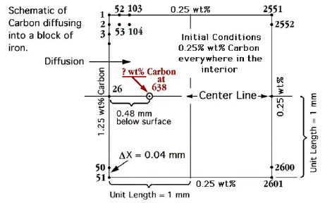
The reason for having unit length and intervals of unit length is so that it is easier to establish the location of the point which is 0.48 mm into the block of iron shown in Fig. 1.

Figure 1. Example Problem 5.2 Geometry ( 51 x 51 mesh dimensions set to determine concentration a point 0.48mm to the right of the left boundary)
The grid dimensions are setup so that a grid point at 0.48mm from the left edge of mesh shown in Fig. 1 can be compared with the result predicted at 0.5mm of the Example Problem 5.2. Location of a grid point at 0.48mm, near 0.5mm, is established by setting up two unit lengths to define the boundaries of the sample where each unit length is 1 mm long. Then 25 intervals are set within a unit length so that each interval is 1/25 th of a mm. Therefore at 12 intervals from the left edge of the mesh boundary a grid point is located at 0.48 mm. As an exercise for the student, a modified grid can be constructed to locate a mesh grid point precisely at 0.5mm. Show two different ways to modify the existing computer program to locate a mesh grid point precisely at 0.5mm.
The original FORTRAN77 / FORTRAN90 programs can be "downloaded" onto a pc and run, but these programs generate data files that require 30 MBytes disk space. In 1995, when this exercise was created, 30 MBytes of disk space was significant. Hence a smaller example problem was created with a smaller mesh size ( 11 x 11). We anticipate that future computers will facilitate larger more realistic mesh sizes. Two different example problems in next section describes how to change mesh parameters for two different meshs. This provides a useful exercise for students interested in modifying the orginial diffusion computer programs.
When increasing or decreasing the size of the grid, shown in Fig. 1, change the value of N. Next change the dimensions on U, UU, ILHS, IRHS, A, B, C, D, E, G, and H according to the relationships described below.
Changiing the size of a square grid, the number of intervals (N) needs to be changed. To calculate N, determine how many nodes along the width of the grid that you want and subtract one and then divide that number by two. The dimensions for UU are just the number of nodes along the width and height of the grid. The dimension on U, A, B, C, D, E, G, and H is the number of nodes along the width of the grid squared. The dimension for ILHS and IRHS is the the number nodes along the width minus two.
When decreasing the size of the grid, change the value for N. None of the other variables need to be changed for the program to work, but in order to conserve space, the dimensions on the variables may need to be decreased according to the relationships above.
A) For example if a 31x31 mesh is desired, then change the value of N=(31-1)/2=15. The dimensions on UU would be (31,31). The dimension on U, A, B, C, D, E, G, and H would be 31*31=961. The dimension on ILHS and IRHS would be 31-2=29. The value for PAR would be 25.4*15^2=5715.
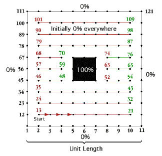
B) In the next example a smaller mesh size of 11x11 is created with inclusions that have concentrations set in the interior. Initial conditions require concentrations that are set to zero everywhere except for a square in the center that is initiailized to 100% concentration on the inclusion boundary, see Fig.2.
In order to change the program to make it match this new grid, some of the initial values of the variables need to be changed. The value for N is 5. The dimensions on the variable UU are (11,11). The dimensions on U, A, B, C, D, E, G, and H is (121). The dimension on ILHS and IRHS is (12), the reasoning behind this will be explained below. The value for PAR is 635. The initial conditions must be changed so that the program reads:
C       PRESCRIBE THE INITIAL CONDITIONS
C
      TD=0.0
      DO 11 IB=1,121
      U(IB)=0
   11 CONTINUE
      DO 12 IB=49,51
      U(IB)=100
   12 CONTINUE
      DO 13 IB=60,62
      U(IB)=100
   13 CONTINUE
      DO 14 IB=71,73
      U(IB)=100
   14 CONTINUE
This will tell the program the concentration at the starting point.
The statements above also assign values at the interior points so the next three lines:
C       ASSIGNING INTERIOR POINT VALUES
C
         DO 9 JJ=1,M
       9 U(JJ)=0.25
must be removed or the value changed from 0.25 to 100.

Figure 2. Example Problem Grid Geometry
According to the rules above, the arrays ILHS and IRHS should have a dimension of (9). The obstacle in the center of the grid can be included by adding three extra entries for the ILHS and IRHS arrays. Locations of these extra entries are easily determined by inspection in Fig. 2. as : point numbers 52, 63, 74 for ILHS and 48,59,70 for IRHS. This means that the array dimension of ILHS and IRHS needs to increased to (12). The boundary conditions need to be changed so that the program now looks like this:
C       LOCATING BOUNDARY AND ASSIGNING VALUES
C
C * indicates new values that define obstacle boundaries
C LEFTHAND#s, Red         RIGHTHAND#s, Green
      ILHS(1)=13               IRHS(1)=21
      ILHS(2)=24               IRHS(2)=32
      ILHS(3)=35               IRHS(3)=43
      ILHS(4)=46               IRHS(4)=48 *
      ILHS(5)=52 *             IRHS(5)=54
      ILHS(6)=57               IRHS(6)=59 *
      ILHS(7)=63 *             IRHS(7)=65
      ILHS(8)=68               IRHS(8)=70 *
      ILHS(9)=74 *             IRHS(9)=76
      ILHS(10)=79              IRHS(10)=87
      ILHS(11)=90              IRHS(11)=98
      ILHS(12)=101             IRHS(12)=109
Here we have designated the ILHS numbers as red and the IRHS numbers as green so that
the reader can more easily identify these points in Fig. 2. The ILHS and IRHS boundaries
provide a limit where as each iterations scans through this mesh, the boundary values
are only seen as N, E, W, or S points.
When additional boundary points are defined in the interior, calculations in Subroutine SLEEP require that an additional start at point 13 is needed to avoid the obstacle where the ninth statement in subroutine SLEEP needs to be changed. The loop in subroutine SLEEP needs to be changed from 1 to NM + 3 to include the three additional scan lines, which are highlighted in Fig. 2 as three green lines, that start at points 52, 63 and 74.
   OLD:   DO 3 J=1,NM
   NEW:   DO 3 j=1,(NM+3)
NOTE: This technique should also work for any irregular shaped obstacle.
With these changes the program will now generate output that can be converted into another movie. But because of a time to complete this project we only show images of concentration at the Initial Conditions and a radial symmetric gradient of concentration of the Steady State Conditions when time goes to infinity.
Larger grids, e.g. 51x51 nodes, will give better results where images will show a more continuous gradient in concentration, but this would require more cpu time and disk storage for larger files. We recommend that students start with smaller meshs. With the advent of cheaper higher performance desktop computers we anticipate that students will want to modify these example problems to include larger meshs and more complex geometries, e.g. multiple inclusions. Modifications to include inclusions was largely motivated to model diffusion of drugs through human skin, where unlike diffusion of carbon through iron, the diffusion of drugs through human skin will require a composite model of inclusions that will not absorb drugs and act as diffusion barriers.
Because these programs are REALLY old, back in 1971 when this program was first written, memory was limited to less than 64,535 single precision words. Hence a code fragment defining a dimensioned array, A, would look like ...
DIMENSION A(65535)
This serious limitation had a lot to do with how programmers wrote their code. In the example FORTRAN code a one-dimensional (1D) array, U(2601) was used for calculations and the 2D array UU(51,51) was added later for archiving data used for post-processing animated 2D graphical plots. Today (2004) even desktop computers have very large memory capacity and 2D and 3D arrays are preferred when working with 2D and 3D finite difference grids on parallel computing systems. It is recommended that the example FORTRAN programs be rewritten and use only 2D arrays.
End of Numerical Implementation of Finite Theory: with examples in diffusion.