PROCEDURE
Motivation
After the optimization process using the Sensitivity Equation method (SEM), the user obtains as a result from the combination of the optimization and the flow solver, the optimal shape of the airfoil (body), the Euler or Navier Stokes solution to the flow and the sensitivity values for the flow at the design point. Frequently designers are interested in the flow around the optimized body for stream condition different than the design conditions. It has been shown that for small peturbations from the design point, the flow can be approximated by a Taylor series according to the formula
where Q represent the primitive (conserved) variables of the flow, a is the peturbed parameter and the partial derivative represents the sensitivities. Examining the flow around the body for conditions other than the design conditions may yield regions in the operational space with unsatisafctory performace. That will aid the design process by eliminating design with poor overall performace.
Objective
Objective of this project was to develop a visualisation tool in which a designer can peturb some parameter of the flow and obtain very fast the new flow. When the reference flow is given along with the sensitivities for that flow then all it is need to obtain the new flow (Taylor series approximation) is a matrix multiplication (sensitivity) with a scalar (peturbed parameter) and a matrix additon.
Tools
In the visualisation class of Pr.of. R. Kriz we learned several visualisation tools. At the beging AVS (Advanced Visual Systems) was selected as the platform to develop the application. Because of the poor performance of AVS in 2D graphics (exelent performance for 3D graphics) soon we made the desicion to choose PV-WAVE as the platform to develop the application.
Formulate the problem
The first case considered with the new developed visualitation tool was that of a flow around the airfoil. The data (optimal airfoil,flow and sensitivities) were generated by the software package LaRC developed by Dan Somers, which couples a flow solver and an optimization algorithn, and were provided by Dr. Andy Godfrey who works for AEROSOFT and Dr. E. M. Cliff Mentals Reynolds Proffessor at Virginia Tech. Because both the flow solver and the optimization algorith were designed to solve 3D problems the data provided were pseudo 3D data with the data in the xy palne being repeated iin the z-direction.
Data
The above descibed data were provided in three ASCI-files (plot3D format) :
- The first file contained the grid data, that means the geometric possition of the grid nodes. In the example case present here the grid was a three dimensional C-grid.
- The second file contained the flow solution around the airfoil (wing).
- The third file contained the sensitivities with respect to the angle of attack (AoA).

The way the data are organized in the ASCI
files provided is :
First all the x-coordinates of the nodes
for all the three planes are stored. Then the y- and z- coordinates
follow. The organitation of the data in the flow solution file and the
sensitivity file is similar. The order of the five different recorded variables
is : Density, velocity component in the x direction, velocity component
in the y direction,velocity component in the z direction and pressure.
The original grid extens to a wide region
compared with the lenght of the airfoil which is one meter. Since the real
intresting flow variations occur in the region close to the airfoil, as
a first step in order to increase the processing speed of the application
we croped the grid to contain only the interesting regions. The croped
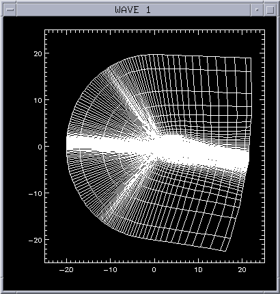
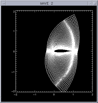
grid is depicted in the following figure :

The data reduction achieved by croping the grid was 40%. Note that the data used in all the subsequent figures and the example fdownload-files are for the sensitivities calculated for an airfoil at an angle of attack of 4 degrees with Ma=0.5 and Re=0.5*10^6. In the following chapter we will provide a user manual for runing the program.
procedure.html