ESM4714
Scientific Visual Data Analysis and Multimedia
Exercise #7: AVS-Introduction
Example:
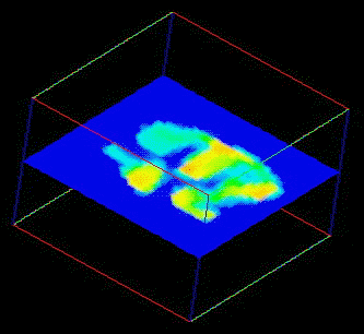
4D Volume Visualization of Fluid Physical Properties
Example: Setting up and using AVS in the CAVE
NCSA has an excellent
AVS tutotial that was created by John Shalf
who was a former Virginia Tech student who took this course in 1993.
Example: 4D Volume Visualization of Fluid Physical Properties
NOTE: Highlighted italic text denotes user response.
Objective:
Understand how to setup a visual paridgm for extraction of physical property relationships
Procedure:
- Logon onto mercury -> pluto.smvc.vt.edu at the VT-CAVE classroom (SMVC).
- Mount your optical disk (see procedure for mounting scsi devices).
- Go to the ESM4714/examples directory.
- Locate files D.fld (density), P.fld (pressure), and T.fld (Temperature), in the
directory
/optical/ESM4714/examples/ragab/viz_method/gas/fields/. The field file
D.fld is listed below as an example.
# AVS Field File
#
# 3D Density
ndim=3            #number of dimensions in the field
dim1=73           #dimension of axis 1
dim2=129          #dimension of axis 2
dim3=73           #dimension of axis 3
nspace=3          #number of physical coordinates
veclen=1          #number of elements at each point
data=integer      #data type (byte, integer, float, double)
variable 1 file = /optical/examples/ragab/viz_method/gas/
D.file filetype=ascii
NOTE: you may have to change the path in the last statement
if you are not using your optical disk.
where ndim=3 defines a 3D field, dim1, dim2, dim3 are the original dimensions of
the Ragab data set, nspace=3 defines the number of physical coordinates, veclen=1
defines the vector length or number of elements assign to a property at each of
the coordinate points (for a vector such as a velocity veclen=3 which corresponds
to the three x,y,z components of velocity), the data type is integer, and the
field type is uniform, and finally the path to where the original ascii integer
data file was stored.
Create the same type of field file for the brown data set and call it C.fld and put it in the brown directory.
#AVS Field File
# 3D Concentration
#
ndim=3
dim1=64
dim2=64
dim3=44
nspace=3
veclen=1
data=integer
field=uniform
variable 1 file = /optical/example/brown/brown.ascii.start filetype=ascii

NOTE: you may have to change the path in the last statement
      if you are not using your optical disk.
Execute AVS: viz?% avs --> a window should appear on the left of the screen.
Choose (click left mouse button) the window 'network editor' --> a larger
window will appear on the right with modules at the top.
- - Choose the "readfield" and "generate colormap" modules from the "Data
Input" section of the module library by dragging (holding down the left mouse
button and moving simultaneously) these modules into the empty window below.
Continue this process by also dragging modules "field to byte" from "filters",
also drag "arbitrary slicer" and "volume bound" from "Mappers" and finally drag
the module "geometry viewer" from "Display Output" where you can place these
modules in a pattern similar to that shown below.

- - To connect modules, move the pointer into a color tabbed region on the
perimeter of the module: red is for output to an image module and blue is for
data. For example the blue region of the "read field" module is connected with
the blue region of the "field to byte" by holding down the middle mouse button on
either of the two tabs until a thin blue line appears and is seclected by moving
the mouse until the thin blue line changes to white and the mouse button is
released and then the white line become the final inforamtion path. Continue to
connect the remaining modules: blue to blue, red to read, and yellow to yellow,
etc.
Data is read by the "read field" module by selecting the small square in the
"read field" module with the left mouse button and a window appears at the left
from which a file is selected with the right mouse button and directories are
also selcted with the right button touching the top most "/" in the window.
Experiment with the various controls until the usage becomes clear. Most of the
choices are intuatitive.
You can observe the flow of data from module to module. When the data
enters the last module ("geometry viewer") an image appears in a window which
should look familiar.
Sometimes the image in the window is too big. To shrink the image to fit
inside the window, press the shift key followed by the holding the middle mouse
button down and dragging the mouse pointer from the top of the viewing window to
the bottom until you get the desired image size. Now let go of the shift key and
grab the edge of the image with the middle mouse button and rotate the image into
desired orientation.
Experiment with moving the arbitrary slice. Choose the slicer controls by
clicking on the small square on the right side of the "arbitrary slicer" module:
the slicer controls will appear in the window on the left. If you decrease the
resolution in the plane the slice moves faster but the images is more coarse.
Try other features such as the "isosurface" module.
Example: Setting up and using AVS in the CAVE.
Like NCSA, Virginia Tech also installed AVS on the VT-CAVE computer.
VT-CAVE has also installed a real-time AVS to CAVE link called
GROTTO viewer (AVS cave_viewer network module) that was created at the
Naval Research Laboratory's Virtual Laboratory
.
Below we provide a brief description on how to used AVS in the VT-CAVE.
Procedure: Viewing the brown.ascii.start data set in the CAVE
- Logon onto the VT-CAVE (contact R.D. Kriz for procedure to get a CAVE
account)
- If you have an optical disk, mount your optical disk (see procedure for mounting scsi devices).
- Contact the CAVE Sysadmin and have them install the .grottorc file
in your home directory.
- Find and change directory to grotto_viewer setup on rkriz's home directory.
To setup a similar grotto_viewer in your home directory contact rkriz@vt.edu.
- cave% cd ~rkriz/NRL_grotto/grotto_viewer
- Start up AVS.
- cave% avs -size 1024x768
- Proceed to build the same network as described in the previous procedure
in steps 8 thru 9. From the read field module locate and select the
same C.fld file you created on your optical disk in step 6. After you confirm
that the network module is functioning correctly, follow the procedure below
to view the results in the CAVE.
- In the upper left corner of the AVS Network Editor window select
Module Tools and just below that select Read Module(s). Another
window will appear from which you can select the file named grotto_viewer.
You will notice that when selected grotto_viewer appears as a module in the
Data Output section of the Network Editor.
- Drag the grotto_viewer module into the network programing area and
connect it to the other modules as you did with the geometry viewer
module ---- a new window will appear near the center of the CRT screen. Drag
and move this window to a convenient location by holding down the alt+f7 keys
with the mouse cursor located over the window and hold down the left mouse
button and drag the window a new location.
- NOTE: The middle mouse button rotates image and the right mouse button zooms in and out. The window generated by the geometry viewer module uses
the standard AVS mouse format.
Example 2: AVS used to view molecular dynamics simulations.
AVS is used closely with supercomputer simulations. For a summer project
in 1995,
Michael Yilma (NSF Summer Undergraduate Research Program), created a
Tutorial on
Molecular Dynamics which used AVS to view the motion of small group
of atoms. Since the number of atoms was small the calculations can be done
on a PC computer. The tutorial was designed so that all information could
be downloaded and simulations done on a remote site computer and the results
of the simulation transfered to workstations in the SMVC and visualized with AVS.
 Click image to return to Visualization home page.
R.D. Kriz
Virginia Tech
College of Engineering
Revised 01/10/99
http://www.sv.vt.edu/classes/ESM4714/exercises/exer7/exer7.html