Figure 1. The LCS
by
Doug G. Gaff
ESM 5984 Final Report
9 May 1995
The term "machine learning" is used to describe a vast array of algorithms, methods, and paradigms which attempt to solve tasks that run the gamut from speech recognition to financial analysis to robot control. Machine learning paradigms tend to fall into one of three categories: neural modeling, symbolic concept acquisition, or domain-specific learning [5]. The neuron-like networks present in neural modeling techniques provide fast, relatively simple mappings from input to output. Symbolic concept acquisition encompasses a broad range of artificial intelligence methods in which a machine solves a task by learning previously unconnected concepts using a predefined symbolic notation. Domain-specific learning involves a large amount of a priori knowledge about the task, and these algorithms focus on using an extensive knowledge-base to solve the problem [6]. In attempting to solve a particular task, one would often prefer an approach that provides a compromise between these three techniques. The Learning Classifier System (LCS) proposed by John Holland [3,2], provides such a compromise.
The LCS is a rule-based, message-passing, machine learning paradigm designed to process task-environment stimuli, much like the input-to-output mapping provided by a neural network. In addition to neural-like mapping, the LCS provides learning through genetic and evolutionary adaptation to changing task environments. LCS concepts are "subsymbolic," meaning that they are encoded by the system itself and not the designer. The LCS can still be programmed with specific domain knowledge, however, and this duality provides much design flexibility [1].
The purpose of this document is to briefly describe the learning classifier system and to illustrate a parameter optimization that enhances its operation. The LCS is applied to a robotics application known as the animat problem. We will show that with scientific visualization, one can optimize the solution to the animat problem.
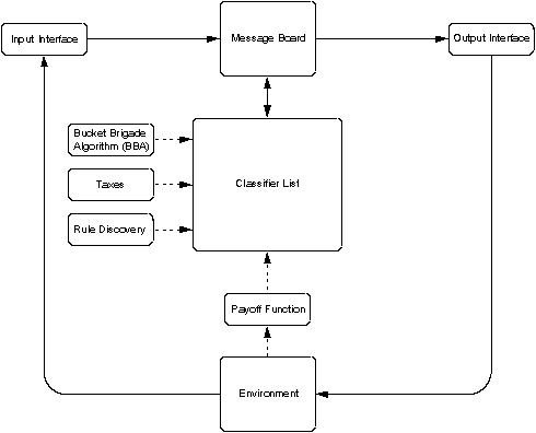
The learning classifier system consists of a list of rules or classifiers that provide a set of possible actions for a given problem scenario. Each rule has one or more condition words and an action word. The system operates by reading messages from a task environment interface, comparing those messages to the conditions of the rules in the classifier list , and posting the corresponding action messages back to the task environment. This sequence of operations is referred to as an execution cycle and is repeated until a particular environment state is reached. Messages from and to the environment are stored on a message board. Since the message board is of finite length, rules are probabilistically selected using a bidding process based on a figure of merit called strength. Each rule has a strength assigned to it, and rules whose conditions match the environment messages are given a bid value based on this strength. Rule strengths are adjusted by the task environment payoff function based on the appropriateness of the rule to solving the task at hand. Rule strengths are also adjusted by the Bucket Brigade Algorithm (BBA), an algorithm designed to encourage rule chaining. Rule chains form when an action message from the previous iteration of the execution cycle causes an action to get selected on the current iteration. In order to provide a method for exploring new rules, the rules in the classifier list are periodically modified by a genetic algorithm (GA) which employs the reproduction and mutation genetic operators. The combination of the GA (rule discovery) and rule strength adjustment ( credit assignment) enable the LCS to learn new concepts. Credit assignment and rule discovery are performed after actions are posted to the environment. In addition, the LCS keeps a "check" on the wealth of the system by periodically applying taxes to the rule strengths. A block diagram of the LCS is shown in Figure 1. The solid lines represent the flow of messages in the LCS, whereas the dotted lines represent internal control, such as rule discovery and credit assignment. For a more detailed discussion of the LCS, see [3] and [2].

Figure 1. The LCS
In order to test and characterize the learning classifier system, we apply the LCS to a particular robotics task known as the "animat problem." The animat problem consists of a simple, autonomous robot, called an artificial animal or "animat," that is put into an obstacle-filled environment [7]. The animat must maneuver around obstacles and reach a goal with the help of some sort of control mechanism. For our discussion, we use the LCS as this mechanism. Essentially, the LCS will function as the "brain" of the robot, thereby selecting robot actions based on sensor information.
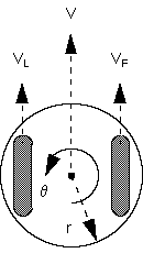
The animat is realized by a treaded robot subject to the nonholonomic constraint. This constraint states that the robot's velocity is limited by its position, thereby requiring that the robot travel only in the direction in which it is pointed. Such a robot is illustrated in Figure 2.
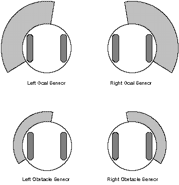
In addition to having a treaded movement, the robot will be able to sense goals and obstacles within a certain sensor range, as well as determine relative directions and distances to them. Sensing will be accomplished using arrays of infrared and ultrasonic sensors. The robot will have left and right sensors for both goals and obstacles, and the angular detection region of these sensors will overlap slightly in the middle to indicate a goal or an obstacle directly in front of the robot. Also, the distance range of the goal sensors will be much larger than that of the obstacle sensors. Figure 3 illustrates the animat sensor model.
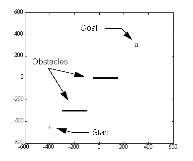
The first facet of animat simulation is to devise a challenging scenario for the robot. This scenario must provide both obstacles for the robot to maneuver around and a goal to be reached. Figure 4 shows the typical "playing field" to be used in the animat simulations. The field is infinite in length and width and contains a goal and two long obstacles near the field's origin. While all units are dimensionless, it is helpful to think of all distances and lengths in centimeters. The robot starts in the left-hand corner of the field at (-400,-450) and attempts to reach the goal at (300,300).
To interface this environment with the learning classifier system, the input and output interfaces must be defined. The input interface reads the four sensors shown in Figure 3 and translates the sensor information into the binary word format used by the LCS. The output interface takes the action selected from the classifier list and translates it into one for four possible robot actions: move forward, stop, move left, or move right. In order to evaluate the decision made by the classifier list, the environment payoff function tests three conditions to determine the rewards and penalties: distance to goal, angle to goal, and obstacle crash. Rewards are given if the robot moves closer to the goal or points more directly at the goal. Penalties are given for the converse of the previous and for crashing into an obstacle. The payoff function is therefore:

where fg, fφ, and fc are flags indicating closer to the goal, pointing more at goal, and obstacle crash, respectively. Wg and Wφ, are reward amounts, and Pg, Pφ, and Pc are penalty amounts. In our simulations, Pg and Pφ are set to half of their corresponding reward values. Note that crashing is always penalized.
The environment payoff function given above has a large amount of influence on how effective the LCS is at controlling the robot. The function has five payoff quantities: Wg, W, Pg, Pφ, and Pc. In order to simply the function, we set the distance and direction penalties to one half of their corresponding reward values. Therefore, environment payoff is a function of only three independent parameters: the distance to goal reward Wg, the direction to goal reward Wφ, and the crash penalty Pc.
Since the purpose of the animat problem is to reach the goal in the minimum number of clock ticks, we would like to find an optimal combination of payoff values that provides this minimum. For the simulation presented in this section, we have performed a parameter sweep over the three independent variables of the payoff function. This parameter sweep can be visualized as a four-dimensional data set, where the first three dimensions are the independent variables, and the fourth dimension is the number of iterations N for that particular combination of rewards and penalties:

Graphically, we can visualize this data set as a volume of varying density, where each dimension of the volume is a payoff quantity, and the densities are the number of iterations for a particular combinations of payoffs. For the simulation, we vary Wg , Wφ, and Pc from 0 to 10 in steps of 1. We therefore get a data set consisting of 113 = 1331 points. For each point in this set, we run ten simulations, each with a different random seed, and average the results.
We use color to represent the number of iterations, where the colors toward the purple end of the spectrum represent the smallest number of iterations and hence the best solutions. We set the maximum number of iterations to 2000, but choose a color range up to 1000 to improve the resolution of the lower end of the scale. In figure 5, we show an iso-surface for parameter combinations which result in N 350. The minimum number of clock ticks for this data set is approximately 188, and this minimum occurs when Wg= 1.0, Wφ = 1.0, and Pc = 3.0. However, as can be seen from the figure, there are several good parameter combinations, most of which have larger goal and direction rewards and a small crash penalty. This result implies that the crash penalty is not as useful in the particular obstacle environment used for these simulations. However, in an environment cluttered with obstacles, a crash penalty might prove to be more useful. For comparison, we have also included a worst-case iso-surface for parameter combinations which give N 500 in Figure 6. We give sample animat paths for the best and worse case scenarios in Figures 7 and 8.
Finally, we should point out that the minima shown in the iso-surface of Figure 5 are only local minima. Several other LCS parameters were held constant in order to generate this plot, e.g. classifier list length, message board length, bid constant, etc. If we were to change these parameters or enable the genetic algorithm, the minima could possibly shift.
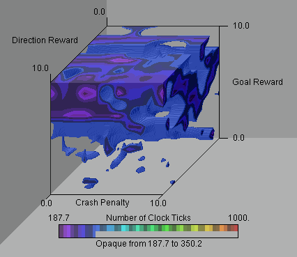
Figure 5. Iso-surface for good parameter combinations
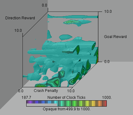
Figure 6. Iso-surface for poor parameter combinations
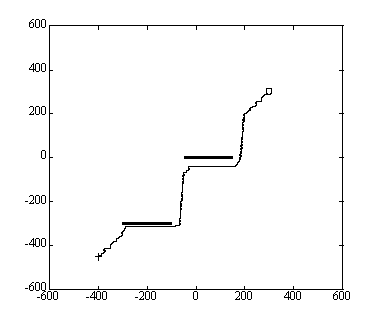
Figure 7. Animat path for good parameter combination ( Wg = 7.0, Wφ = 8.0, Pc = 1.0)
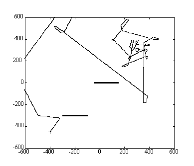
Figure 8. Animat path for poor parameter combination ( Wg = 2.0, Wφ = 1.0, Pc = 9.0)
Through the use of scientific visualization, we can take a large data set and examine its characteristics, thereby arriving at conclusions not readily evident by normal analysis techniques. In the parameter optimization presented here, we were able to conclude that the goal and direction rewards are much more important than the crash penalty for the success of the animat in an obstacle-filled environment. The iso-surfaces suggest that we may wish to eliminate the crash penalty completely, and possibly enhance the payoff function with another parameter. For example, we might add parameter to the payoff function that rewards the animat for moving away from obstacles, rather than penalizing it for crashing into them.
[1] Belew, R.K., Forrest, S., "Learning and Programming in Classifier Systems" in Machine Learning Vol. 3, Boston: Kluwer Academic Publishers, 1988.
[2] Booker, L.B., Goldberg, D.E., Holland, J.H., "Classifier Systems and Genetic Algorithms," Artificial Intelligence, vol. 40, nos. 1-3, September 1989, pp. 235-282.
[3] Holland, J.H., etal., Induction: Processes of Inference, Learning, and Discovery , Cambridge: MIT Press, 1986.
[4] Huhns, M.N., Distributed Artificial Intelligence, California: Morgan Kaufmann, 1987.
[5] Michalski, R.S., "Understanding the Nature of Learning: Issues and Research Directions," in Machine Learning: An Artificial Intelligence Approach Vol. 2, Boston: Kluwer Academic Publishers, 1987.
[6] Rich, E., Knight, K., Artificial Intelligence, second edition, New York: McGraw-Hill, 1991.
[7] Wilson, S.W., "Classifier Systems and the Animat Problem" in Machine Learning Vol. 2, Boston: Kluwer Academic Publishers, 1987.
Added class project as CVDC case study, October 2007
Original: http://www.sv.vt.edu/classes/ESM4714/methods/Gaff.html
Current: http://www.sv.rkriz.net/classes/ESM4714/methods/Gaff.html