What is Molecular Dynamics?
Molecular dynamics deals with simulating the motion of molecules to gain a better understanding of chemical reactions, fluid flow, phase transformations, droplet formation, and other physical phenomena that derive from dynamic molecular interactions. Scientific visualization is used for understanding the result of a molecular dynamics simulation: How is one to understand the mechanism of water molecules diffusing through a complex polymer structure, recognize the formation of a vortex in the mass of data, or the nature of the bending and stretching of a large molecule? How is one to gain new insights? Pictures and animations enable the scientists to literally see the formation of vortices, to view protein folding, and thus to gain new insights into structure <-> property relationships. Computer simulation provides a direct route from the microscopic details of a system (the masses of the atoms, the interactions between them, molecular geometry etc.) to macroscopic properties of experimental interest (the equation of state, transport coefficients, structural order parameter, and so on.) The tutorial below is designed to introduce the student to the basic elements in modeling and visualizing results. More complex theories build on these ideas.
Before you begin this exercise you should download, MolecularDynamics.ps from our anonymous file server, ftp.sv.vt.edu, and print a copy of the manusctipt "Molecular Dynamics: An Introduction", Lloyd Fosdick, University of Colorado, January 19, 1995 to a postscript printer. You must READ THIS DOCUMENT FIRST before you can understand how to modify the FORTRAN program in the following exercise. This document was created by the HPSC group at University of Colorado (CU) under NSF Grant CDA-9017953. This file can also be downloaded from CU's ftp server, ftp.cs.colorado.edu/pub/HPSC/MolecularDynamics.ps.Z .
In order to complete this exercise, you will need the following files. You can save these files as plaintext to your own directory for later use. Name these files the same as their hypertext names.
There are three different types of models: Hooke's Law (HL), Lennard-Jones (LJ), and Hard Sphere (HS) . Of these three models, the LJ model comes closest to representing real molecular systems. Because the LJ model is also easy to work with in three dimensions (3D), we will work with the LJ model in this tutorial. Even though 3D models are more realistic it may be instructive to start with 1-dimensional and 2-dimensional systems.
Note: If you would like to apply the 1 and 2-dimensional concepts in the LJ model, you will need to modify this FORTRAN Program.
Models of particle systems are characterized by the nature of the interactions between the particles. By going through the following steps, you can create your own LJ model.
When you are ready to experiment with your own input data, click here for description of input file.
NOTE: all UNIX commands are denoted with bold-italic letters and we use the viz2% prompt throught out this procedure, although Step I of this procedure will also work on all other UNIX workstations (viz1, viz5, viz6, viz9 and viz10) in the Laboratory for Scientific Visual Analysis (LSVA) or the Sparc20s (mercury, venus, mars, etc.) in the Scientific Modeling and Visualization Classroom(SMVC). We encourage the student to download programs in Step I and run the simulation using FORTRAN compilers on their own personal computers. To visualize their results with AVS we provide access to UNIX workstation in the LSVA or SMVC. The Makefile used in this procedure will only work with AVS Versions 3.0 (on viz2), or 5.3 (on mercury, venus, mars, etc.).
Note: Remember to change the input and output locations. If you would like to read from "md.in" and store your data to "md.out", make sure the following statements are in your FORTRAN program.
OPEN (UNIT = 2, FILE = 'md.in')
OPEN (UNIT = 3, FILE = 'md.out')
viz2% f77 molec_dyn.f -o molec-dyn.x <return>
or
viz2% f90 molec_dyn.f -o molec-dyn.x <return>
viz2% molec_dyn.x <return> This command will create the store results in the file "md.out"
NOTE: The remaining procedure will only work on with AVS Ver 2.0, 3.0 or 4.0.
viz2% make <return>
This command will execute commands in Makefile and will create an anim_ball_color executable file anim_ball_color.exe
NOTE: make sure Makefile is in the same directory with your anim_ball_color.c program.
viz2% avs <return>.
.gif)
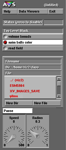
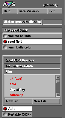
For some reason this window can start in a directory that is not your home directory, therefore you may need to go all the way back to the root directory ( / ) by clicking on the symbol ( .. / ) at the top of the column. Notice that each time you click on ( .. / ) you go backwards in the directory structure. From the root directory ( / ) you can than go forward to your home directory and locate the file anim-ball-color.exe by selecting the appropriate directory names: for viz2, for example, this path would be /home/viz2/class/ etc.
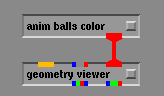
When you find the file anim_balls_color.exe select it by pressing on the left mouse button and you will notice that this module in added, in alphabetic order, at the top of the Data Input column of modules in the Network Editor.
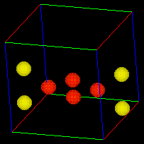
The module anim_balls_color has an additional feature to change the color of each atom. Click here for an explanation of the changes you will need to make on your output file. Different colors are used here to differentiate different types of modal vibrations.
Notice that here Mike Yilma, the author of this execise, has created a directory named "yilma" off of the "class" home directory and has stored the file "md.out" in the directory named "Modules". If you use viz2.sv.vt.edu for this exercise you should create your own directory but remember that when you finish your files may be erased by the next user that logs onto viz2.sv.vt.edu. Therefore if you want to continue to work on your FORTRAN and AVS programs you should work on the mountable optical disk located somewhere near viz2's optical disk drive.
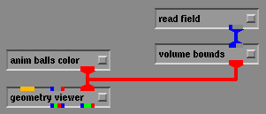
Once the "box.fld" file is selected the bounding box should appear in the geometry viewer window as show below. With this box you can now rotate and change the view angle of the box by using the middle and left mouse buttons without affecting your animation.
This molecular dynamic exercise deals with the LJ model. As we mentioned earlier, the main characteristics of LJ are strong repulsive forces at very short distances between atoms, attractive forces at larger distances, and extremely weak attractive forces at very large distances. We can witness these three types of forces in the eight atom example shown below: 1. The initial vibration of this 8 atom configuration shows that attractive and repulsive forces result in a stable vibration (NOTE: because the governing equations are nonlinear, the vibration is chaotic and exhibits three different stable vibration configurations), 2. The vibrations continue to evolve into a unstable configuration where all the atoms scatter alway from each other and leave the bounding box which is a result of weak attractive forces at very large distances. Use this example input file to create your own 8 atom movie (1.9 Mbyte) and see if you can reproduce these results with your own FORTRAN program.