1.2 Current Drug Delivery Systems
There are advantages and disadvantages to all of the forms of drug delivery listed above. The intravenous method is the best for direct delivery and control of rate of delivery, but it is the worst because it can transmit foreign organisms into the body (highly invasive). The tablet is best for convenience, but its shortcomings are the sudden high rate of release and fast depletion of its concentration. Because the tablet cannot be placed next to the site of interest, most of the medicine is passed through the intestines or flushed out by the kidneys before it is even used.
The TDD system is best known for its non-invasiveness and its placement over the target region. However, it has a long list of areas where improvement is needed. These areas include: slow delivery rates, use of diffusion gradients as the main mechanism for transport, over-doses and under-doses, biological tissue irritation, and its dependence with various non linear biological processes. The rate of initial discharge and the depletion of concentration of medication as seen in Figure 1.2.1.
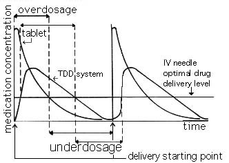
Figure 1.2.1 The concentration of medication in stomach and blood as a function of time, with conventional dosage form.
1.3 Definition of the Problem
The TDD system was chosen as the research topic. The other two methods of delivery are the extremes, one being completely invasive and the other uncontrolled and diluted. The TDD system is somewhere in between, where the risk of transmitting a foreign organism is close to none and the rate of delivery is somewhat controllable. To be able to improve on the design of the TDD system model, we need to study the current model. This model is not well published due to proprietary interests of competing pharmaceutical companies.
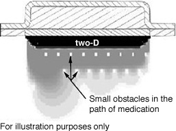
The scope of this project is first to study the diffusion model and then add onto that the other governing mechanisms of transport. Diffusion is defined as the process whereby a material moves from a region of higher concentration to a region of lower concentration, Ref (1). Diffusion in this model will take place starting from the drug reservoir, moving through several layers of filters, and then working its way into the skin. From this point on, the mechanism of transport gets very complex. The research literature and the time limits for this project did not allow for detailed modeling of all processes, although they will be discussed in the future work section of this report. In nature, diffusion occurs in a three-dimensional world. To reduce the computer processing time, a two-dimensional representation is used.
The problem is to define both when the diffusion model is applicable and when it is not, and
where the other processes dominate or compete with diffusion in biological tissue.
There are several different mass transport process occurring simultaneously where one process
may be several orders of magnitude larger than the others.
SECTION 2. THE ANALYTICAL TRANSDERMAL DRUG DELIVERY MODEL
2.1 Formation of a Diffusion Model
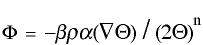
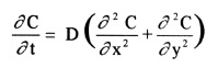
To describe diffusion, one must consider the governing equations, then the different factors that go into controlling mass transport within the human body. The governing equations for diffusion are Fick's first and second law, Ref (2).
Fick's first law can be derived from the Generic Transport Equation (GTE). Fick's first law is derived below starting with the GTE equation:
 [1]
[1]- BETA is the correction coefficient which accounts for the semi-permeability of the membrane and is equal to 1 for full permeability,
- RHO is the density of the molecule in mass per volume,
- ALPHA is the kinematic mass transport coefficient which is equal to
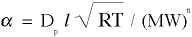 , where
 - Dp is the permeability (i.e., if Dp=1, then the path offers no resistance, or Dp=0 if the path is fully blocked),
- l (lower case L) is the mean free path of the molecule,
- MW is the molecular weight of the molecule,
- R is the universal gas constant, and
- T is the local temperature,
- n exponent on the MW term is set equal to one for this diffusion problem but can also be defined as follows: for mass transport, n=1, for momentum transport, n=1/2, and for energy transport, n=0
- THETA is the intensive potential, the driving force equal which is calcualted from
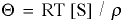 , where
 - [S] is the concentration of species S in units of mass per volume
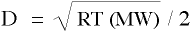
Combining equations yields a relationship that defines the diffusivity, D, of species S as
and redefine variables as follows,
 and
and 
- [S] is the concentration of species S in units of mass per volume
 [2]
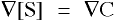
[2]Fick's first law quantifies the amount of matter that is being moved from a point of higher concentration to that of a lower one. The units of mass flux, J, are mass per area per time, the diffusivity coefficient, D, is area per time, and the concentration gradient (grad of C) is mass per volume per unit length.
 [3]
[3]
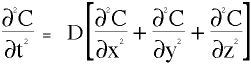
Fick's second law, equation [3], unifies the rate of change of concentration, C, with the
volumetric distribution of the concentration. Fick's laws govern the transport process
from the drug reservoir to the first active metabolic process, for example, the breaking
down of Adenosine Tri-Phosphate(ATP) into usable energy for cellular processes within the
tissue. After the medication reaches the first active metabolic process, an accurate
description of mass transport can no longer depend on the concentration gradients alone.
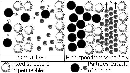
Just as a multiplexer has many inputs and only one output, this transport model has many input variables and one response. This response determines the model's efficiency, speed, order of magnitude, influence over its competition, bio-availibility, metabolic activity, reservoir concentration, and others of lesser importance to the transport taking place. For example, when the heart rate increases, the blood flow rate increases, and, in turn helps to increase the rate of diffusion near the capillary walls due to lower pressures and lower concentrations in that area. However, when the heart rate increases, the rate of heat flow out of the blood also increases, which deters the diffusion process due to the counter convection of water moving radially out of the skin. When the magnitude of the velocity and the pressure are high, the concentration of the diffusing species builds up and the gradient which powers diffusion is nearly zero as can be seen in Fig 2.2.2.
Figure 2.2.2 Shows the influence of built up concentration due to high velocities or high pressure.
Variables that influence diffusion within a tissue include the following:
Just as the human body operates well within its normal operating envelope, mass transport,
which is an integral part of human processes, works well within its ranges.
The scale of matter is very important when considering the diffusion model. On the atomic
scale, there are 3 atoms in an H2O molecule with a molecular weight of 18,
compared to a cell with an average of 10E-14 atoms.
The size of the diffusing species must be equal to or smaller than the largest width
of the pathway. There are two forms of diffusion: vacancy, and interstitial diffusion.
Vacancy diffusion occurs when there is a vacancy of the same size or when another atom
of the same size moves and leaves a vacancy. Vacancy diffusion occurs when you have
impure material. Interstitial diffusion occurs when an atom of the smaller size moves
in-between larger atoms. Interstitial diffusion will occur in materials without
impurities, and in mass transport processes within the human body.
The order of magnitude of the rate of transport will be related to the scale of the
species being diffused and to the scale of the species that it is being diffused in,
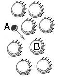
as seen in Figure 2.3.1. For example, the size of a gas molecule compared to the size
of a polymer is very small. So, the diffusive characteristics will be inversely
proportional. The species A (a gas) will easily diffuse through species B (a film)
with a path width greater than or equal to the width of a molecule of species A.
Similarly, species C (a polymer) will not be able to diffuse through a path width
smaller than itself.
Figure 2.3.1 A and B. Influence of relative size/scale on diffusion.
The relative mobility and geometry of the drug molecule will influence its ability
to maneuver around obstacles as shown in Figure 2.3.2 A, B, and C. Rate limiting
membranes (Figure 2.3.2 D) use this mechanism for slowing down the rate of transport.
A particular molecule will have to vibrate and rotate (A->B->C) before it orients
itself in the correct position to pass through the membrane. The rate of transport
will be slower as the membrane geometry gets more complex.
Figure 2.3.2 A, B, C, and D. Influence of Molecular mobility
- Relative convection is the magnitude and direction of the local flow relative to the
concentration gradients. An example of this is cells absorbing or expelling water. If
the cells are absorbing water then the cell walls will absorb the medication into the
cell, increasing diffusion of medication into the local site. When the cells are
expelling water, the excess water will be pumped out of the local area due to
extra-cellular fluid exceeding capacity (i.e. super saturating), this will aid the
transport of medication away from the local area by lowering the local concentration
and increasing the diffusion gradient. However, If this occurs at the target area, the
medication will not be able to move into the cell.
- The heat dissipating mechanism regulates diffusion in the same way as the relative
convection mechanism. This relation is due to the fact that the body regulates its
temperature by regulating blood flow in specific areas. For example, if the body
temperature is higher than normal (37 degrees Celsius), the total percent by volume of
blood heading out to the limbs will increase. The sweat glands will absorb the warm
water out of the blood and move it to the surface of the skin. The water on the
surface of the skin will evaporate, lowering the surface temperature. This process not
only drives the heat radially outward, but it also interferes with any foreign material
trying to work its way in.
- Water aids diffusion indirectly by reducing the viscosity of the fluid medium. The
lower viscosity allows the concentration of the drug to become diluted in this area.
The high concentration of drug at the patch site and the low concentration in this area
generate a concentration gradient directed inwards.
- The metabolic activity rate (MAR) of the local area will control how fast certain
reactions happen. A major foe of diffusion is the active carrier transport mechanism.
The active transport mechanism uses carrier molecules to carry molecules that would
normally not be able to reach their target sites in time for the organism to survive
just by diffusion. An example of a carrier molecule is the hemoglobin molecule, which
binds to it four oxygen molecules. Without the Hemoglobin molecule the blood would only
be able to supply our body with one sixty-fourth the amount of oxygen that it receives
due to Hemoglobin. Molecular binding sites is a major topic for research in the
biomedical field, namely, how to gain access to binding mechanisms on other floater
molecules to get a free ride to the target. The MAR is too fast for any diffusion to
occur. Diffusion is a time dependent mechanism. Two species have to sit next to each
other long enough for diffusion to take place. But if the carrier molecules bind with
and carry away the second species, then diffusion cannot occur.
- As the density of the material increases, its volume for a constant mass decreases,
therefore shrinking the porous pathways that allow diffusion.
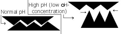
- The pH concentration of the fluid medium controls the speed of the binding reactions
that occur in it. This is done by the secondary bonds and Vander Waals effects. One OH-
will have to repel another OH-, or high pH will not repel its neighbor polymer chain as
much. Normal pH for the human body is 7.4.
Figure 2.3.3 Influence of pH concentration on binding site shape.
The pH controls the shape of a binding site, so that if the pH is just slightly off,
the binding site
is distorted, and the correct binding will not occur as seen in Fig. 2.3.3.
Due to constraints in time and available literature on modeling diffusion that includes active
transport bio-mechanisms, the next section will numerically model diffusion only as it is
influenced by structure. How various active transport mechanisms contribute to the average
diffusion coefficient is currently not known. Hence approximations are made for the diffusion
coefficient used to calcuate concentration gradients in the next section.
Since there is no exact solution for this second order non-homogeneous equation, a FORTRAN
program is used to approximate a solution to this problem. Although diffusion is inherently
a three-dimensional phenomena, only the two-dimensional non-steady state Laplace's equation
is chosen over the three-dimensional equation to reduce the computational work load. To
reduce the three-dimensional equation to a two-dimensional equation, the concentration is
restricted to vary only in the x and y directions, and is held constant in the z direction.
The invariance in the z direction simplifies the three-dimensional equation to the following
two-dimensional equation.
The program developed here, DIFFUSON.FOR, was modified from one that calculated the velocity profile
around a grid (x and y) in time (t). The original program was written by Dr. Ronald Kriz to solve the
same type of equation(a second order, non-homogeneous) to find the velocity profiles around obstacles
within the grid. DIFFUSON.FOR was modified to solve equation [3] with boundary and initial conditions.
This modified program was used as a tool to generate data output for specific materials, and initial
and boundary conditions for MSE2094 (Analytical Methods in Materials Engineering, taught by Dr. Kriz
in Spring semester 1995). More detailed information on the method used to numerically solve equation [3]
can be found in References 5 and 6.
DIFFUSON.FOR reads four input files and outputs one data file. Two of the files read in are
CGATEPOS.INP and FGATEPOS.INP, which input position information for the concentration and the
flux gates. The output file DIFFDATA.OUT, contains information about all of the concentrations,
and an average mass flux for each time step taken within the computation.
The user has control over all of the variables through the input file INPUT.INP,
which defines for the program the following variables:
-N = the number of intervals in one section of the grid, currently set to 99 intervals.
The user can define the number and the size of obstacles for the whole grid by the input file
OBSTACLES.INP. Within the human body, the obstacles can be the different density cell structures
that are encountered along the path of transport.
The output from this program are saved into the file DIFFDATA.OUT. The data in this file are raw and must be processed to be of any value. PV-WAVE, a visualization package, was used for this project in analyzing the output from the FORTRAN program.
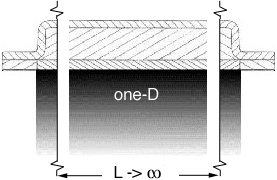
During the beginning of this project, the difference between the one-dimensional
(one-D) differential equation and the two-dimensional (two-D) differential equation
was not well understood. One would have easily replaced the one-D equation with the
two-D equation without much thought of the inherent errors. Through the visualization
of the data output for the one-D and the two-D input conditions, the difference was
observed as in Figure 3.3.1.
Figure 3.3.1 A and B. Shows the difference between the one-D (A) and two-D (B) results.
To calibrate the computer program and its output, Example Problem 5.2 from Callister,
"Materials Science and Engineering", Ref (2), was used as reference. Example Problem
5.2 deals with carbon diffusing into steel. The example problem is a one-D diffusion
problem, but the computer program was designed around the two-D system. One-D and
two-D esults are shown Figure 3.3.1. The left image in Figure 3.3.1 shows an exact
one-D solution and the image the right shows diffusion occurring in two-D. The reason
for the anisotropic behavior is due to the edge effects. To reduce the impact of
edge effects, the width of the grid needs to be increased. If the two-D results shown
on the right were stretched out to infinity they would approach the one-D image shown
on the left. If the width is great enough the percent error between the exact one-D
solution and the two-D numerical approximation at the center point will decrease as
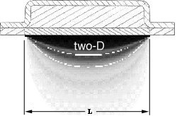
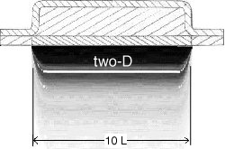
seen in Fig. 3.3.2.
Figure 3.3.2 A, B, and C not to scale, shows the importance of the width of the grid.
Image 3.3.2.A is the result of the one-D exact solution, which is independent of the
width of the grid. Image 3.3.2.B is the result of a two-D numerical solution, where
the grid width is equal to the grid length. Image 3.3.2.C is the result of the same
two-D numerical solution, with the grid width ten time the length of the previous grid.
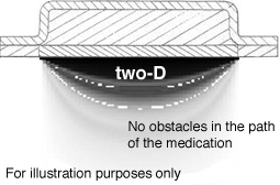
Several different input conditions are tested to show the influence of obstacles in
the path of diffusion. The output form these tests is visualized in Fig. 3.3.3.
Figure 3.3.3 Visualization of the influence of obstacles
Visualization was a tool used in this project to understand the mechanism of diffusion
and allowed us to see how the structure property relationship of a material influenced
its diffusion process.
The model for the transport of medication (from the TDD system to the blood) involves
a lot more than has been described in this report. Due to limited time and resources,
most of the time was spent locating applicable literature. The Virginia Tech Newman
library carries some literature on clinical studies of transdermal drug delivery
systems, but carries none on the detailed mechanics of the TDD systems.
The method of measuring flux in clinical experiments, is obtained from measuring the
concentration of medicine from the urine sample and not directly from underneath the
skin. The computer code for computing flux directly underneath of the skin is included
in this program. But due to the difference in location of measurement, the two values
of flux cannot be compared to each other.
A lot of time was dedicated to the optimization of the FORTRAN program code. The main
problems encountered with the code were: 1) The program used up all available memory
and in some cases locked-up the computer; 2) The output data files were too large to
work with on a PC, averaging sixteen megabytes for one full run (1000 time steps).
A personal computer was upgraded due to the requirements of this project. A UNIX system
gave the most freedom and speed, where an average computation took about ten minutes
compared to four to five hours for the same computation on the PC.
The visualization package, PV-WAVE Personal Edition, by Visual Numerics Inc., was newly
released software for the PC, and it had a lot of problems translating automatic script
files from the UNIX version of PV-WAVE. The best way to work around that problem was to
write and edit the FORTRAN program on the PC, then compile, run, and process the output
on a UNIX workstation. Once the process from initial input to final images is optimized,
one can reach turnaround times from input conditions to full scale movies within ten
minutes. The Scientific Visualization Lab in Hancock Hall was used for optimal results.
The FORTRAN program used a finite-difference method that computed iteration by iteration
in a serial order, i.e. compute information at node-one, then node-two and so on. There
is a more complex FORTRAN code referred to as FORTRAN-M, which computes the node
information for all the nodes simultaneously. The information on this code can be found
at Dr. Hienkenschlos'ss Math 4445 Homepage, in the Math Department.
The FORTRAN program described above simple homogeneous diffusion model. When the other
models of transport are quantified and can be solved, the resulting data output may be
combined with the data output from this process and a morfe complete description of the
transport mechanism in the human body can be developed and studied.
Currently, there are only few medications that can be delivered through the use of the
TDD system, due to the slow rate of delivery. They are: nitroglycerin(for angina-heart
disorders); estradiol(for hormone imbalance); nicotine(to quit smoking); and medications
for infants (infant skin is much more permeable than adults).
When all the mechanisms governing the transport of medication through the skin are fully
understood, we will be able to generate better medications that will move easily through
the barriers of the skin and be delivered to the target location.
Thanks goes to the advisors, Dr. Ronald D. Kriz and Dr. Daniel J. Schneck, for their
continuous support and patience throughout this project, and for the access and use of
the Lab for Scientific Visualization. My appreciation goes out to my classmate and
good friend Kenneth Venzant, my roommates Robert Hunter and Dennis Osgood, and Dr. Eric
Pappas for their help on the style and structure of this report. Last but not least,
thanks to my parents (and my brother, but only for the use of his new computer), who
made all of this possible.
Sanjiv D. Parikh
- Physical scales and geometry;
- Temperature (the process of transporting heat out of the blood interferes with transport of medications into blood);
- Tissue's humidity (water saturation);
- Current metabolic rate (how fast the body is processing food, energy (ATP), and waste products);
- Chemical interactions (competing reactions block pathways where diffusion could occur);
- Time availability (species A and B have to be next to each other long enough for diffusion to take place);
- Density (high densities reduce open pathways and interstitial space);
- pH (has control over processes that interfere with diffusion);
 B
B 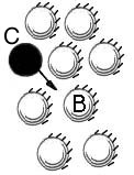
 D
D 
 [4]
[4]
-LVERT = the number of sections on the vertical side of the grid, currently set equal to 1.
-LHORZ = the number of sections on the horizontal side of the grid, currently set equal to 1.
-W = convergence factor for successive over-relaxation (sleep) method, currently set equal to 1.85.
-SIGMA = the constant in the Laplace equation. For our case it is the material diffusivity, set
equal to 1.6*10E-5. This controls the speed of the rate of diffusion.
-THETA = for guaranteed unconditional stability, 1/2 < THETA < 1, currently set equal to .75.
-PAR = this parameter controls the stability of the convergence of the calculation, currently
set equal to delta t times N squared. See Appendix A for details about this parameter.
-TS = total number of time steps, currently set equal to 1000 steps.
-ITMAX = The largest number of iterations for convergence for each time step, currently set
equal to 100 iterations.
-ERRSOR = the percent error to expect in the final solution, currently set equal to .001.
-CONINI = the initial concentration for the whole grid, currently set equal to 25.0.
-CONOBS = the fixed concentration of the obstacles. Work is in progress to make this a variable
(function of time or temp, etc.), currently set equal to 25.0.
-MEDCON = the fixed concentration of medication on the surface. Work is in progress to make this
a variable (function of time), currently set equal to 120.0.
Work is in progress to present the output of several different initial and boundary
conditions with different obstacle geometries. When the resulting image sequence is
captured and collected, and converted into movies that will
show the diffusion process as it occurs for different configurations.
1. Bronzino, J., Handbook of Biomedical Engineering, CRC Press, NewJersey, First Edition,
p.70, 469 (1995)
2. Callister W., Jr., Diffusion, Materials Science & Engineering, An Introduction,
3rd Edition, John Wiley & Sons,Inc., p.97 (1994)
3. Schneck, D. J., The Transport of Mass, Energy, and Momentum in Physiologic Systems,
Mathematical and Computer Modelling, Pergamon Press, New York, NY, Vol. 12, No. 12,
pp.1473-1485 (1989)
4. Carnahan, B., Luther, H. R., Wilkes, J.O. Applied Numerical Methods. John Wiley &
Sons, Inc., New York, p.451 (1969)
5. Kriz, R. D.,
MSE2094 Diffusion Project: Theory of Finite Difference Models with Applications in Diffusion,
http://www.sv.vt.edu/classes/MSE2034_NoteBook/MSE2034_kriz_NoteBook/diffusion/diffintro.html, (spring 1995)
6. Kriz, R. D. and Patel, M.,
MSE2094 Diffusion Project: Numerical Implementation of Finite Difference Theory with examples in Diffusion,
http://www.sv.vt.edu/classes/MSE2034_NoteBook/MSE2034_kriz_NoteBook/diffusion/numeric/numeric1.html, (spring 1995)
If your have any questions you can contact Sanjiv Parikh
at: engineer@vt.edu
College of Engineering
Virginia Tech