|
In order to get the real picture of an orbit, we have to see it in three-dimensional
coordinate space. The most common reference system for the earth
orbiting bodies is the geocentric-equatorial earth coordinate system (see
Basics). For this system, there are six
orbital variables that can produce a vast number of orbits with different
shape, size, position and orientation. I wrote a MatLAB program that
will enable the user to visualize the orbit in three dimensions and hopefully
be useful as a tool in developing a better understanding the effects of
each one of the orbital elements.
The program begins by prompting the user for the six orbital elements described
in the Basics. As in the 2D program, the
user can choose the default values by just pressing the enter key.
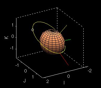
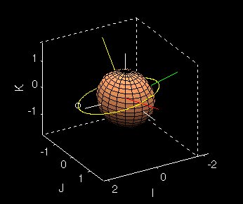
After the user enters the orbital elements, they are given the option of
displaying the IJK vectors on the earth (bottom right figure). The
figures below both contain the earth (copper sphere), the 'P' (red), 'Q'
(green), 'h' (yellow) vectors, and the path and position of the orbit as
in the 2D program. |