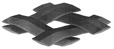
Figure 1. Plain weave composite structure
In engineering and the sciences many examples exist where visual tools have been effectively used by researchers to study massive-complex data sets generated by supercomputer simulations or computer controlled experiments. With visual tools our data-rich but information-poor environment is transformed into an information rich workplace where we can be better scientists, engineers and designers. Greater access to computer resources in all disciplines has prompted users to go beyond the "number crunching" paradigm and establish visual methodologies that are discipline independent. Visualizing gradients in scalar properties (zeroth order tensors) and various types of stress glyphs (second order tensors) are the most popular visual tools. Common to most of these studies is the eigenvalue problem whose eigenvalues (zeroth order tensors) and eigenvectors (first order tensors) can be used to characterize physical properties that are second, fourth, and higher order tensors. A review of visual methods used in mechanics and material science is extended to include fourth and higher order tensors. Here we show how materials researchers can use these visual methods to study residual stresses and cure properties related to complex three-dimensional composite structures. Higher order tensors are used to characterize material anisotropy. The need to study the distribution of tensorial properties in a continuum leads to the development of a visual method that can be used to study tensor equation invariance. This visual method can be used to extract simple functions from "raw data": massive data sets resulting from numerical simulations, computer controlled experiments or both. Unique to this manuscript are enlarged image formats, animated movies, and electronic mail dialogue that can be accessed with a web browser at http://www.sv.vt.edu/NCSA_WkShp/kriz/WkShp_kriz.html . With these new features the authors hope to communicate additional information that will make reading this manuscript a data and information rich experience. Publications no longer need to be a static archival experience: please send your thoughts, comments and critique to R. D. Kriz at: rkriz@vt.edu
In physics, engineering, chemistry, and the other physical sciences the eigenvalue problem is frequently encountered. Structural design engineers encounter the eigenvalue problem when determining the principal stress state in deformable bodies. In fluid dynamics, solutions to eigenvalue problems result in Reynolds stress tensors and the rate of deformation tensors that are used to study fluid particle motion through Eulerian space. Wave propagation in anisotropic materials results in a complex eigenvalue problem that yields homotopy wave velocity surfaces and singularities in particle displacement vibration directions. Although these are all different physical systems, they all have one thing in common: the mathematical model of the physical system typically results in an eigenvalue problem whose eigenvalues (zeroth order tensors) and eigenvectors (first order tensors) represent physical properties that are second, fourth, or higher order tensors. Often these eigenvalues - eigenvectors are embedded in much larger and more complex systems where it is possible to visually isolate these properties as glyphs while observing the glyph's relationship to the surrounding functional space from which they were extracted. The relationship of the isolated glyph to its surroundings can be accomplished by superposition of additional information, typically scalar properties (zeroth order tensors) onto the existing glyph surface. For example the magnitude of the local or convective component of the comoving derivative of a property associated with a fluid particle could be represented by color mapped onto the strain rate glyph moving through Eulerian space.
Visualizing gradients of scalar quantities (zeroth order tensors) has been the most popular visualization technique used to date. Based on the complex textile geometries predicted by Pastore et al. [1], Glaessgen et al. [2] showed that damage resulting from large residual thermal stresses could be studied when three-dimensional gradients of strain energy density were visually superposed onto a representative volume element of a woven fabric-reinforced polymer composite. MacRae et al. [3] showed that another visual approach could be used to study scalar properties associated with cure simulations of resin infusion into a graphite fiber preform. The study of these problems may benefit by the use of glyphs that characterize gradients in stresses and material stiffnesses that are also influenced by the same processing parameters.
This study starts with visualizing scalar gradients and then continues with the construction of a simple second order stress tensor glyph by showing the relationship between the eigenvalue solution to the principal stress state and the shape and orientation of a quadric surface, Fredrick and Chang [4]. Rarely do eigenvalue - eigenvector properties occur as isolated events in a multivariate physical system. Because these properties exist in a continuum of connected properties, Haber [5] and visualization programmers at NCSA [6] represented stress gradients by icons located near a stress singularity of a moving crack tip. Since it may also be important to show the continuity and transition of stress along a trajectory, Hesselink et al. [7,8] have created a visual hyperstream of connected glyphs where two of the three eigenvalues define the shape of a continuous tube and the magnitude of the third set of eigenvalues along the trajectory is mapped onto the tube as a color gradient. Recent visual experiments by Moore et al. [9] have devised yet another glyph for a Reynold's stress tensor whose shape is most useful in studying turbulent flow. The present study extends the idea of visual representations of eigenvalues to tensors of fourth order where it is possible to characterize and study changes in material anisotropy. Most importantly the idea of visualizing tensor quantities in a continuum is extended to the observation of the invariance of tensor equations. This idea is then used to extract relationships from "raw data": massive data sets resulting from numerical simulations or computer controlled experiments.
This section gives two examples of visualizing three-dimensional gradients of scalar quantities that are found in complex composite structures where rheological flow, cure, and residual stresses coexist. In both cases researchers have benefited from visualizing gradients in strain energy density, temperature, pressure, and degree of cure.
When possible, composite materials research engineers seek relationships between material structures, constituent properties and the resulting mechanical characteristics of the composite. If these relationships are understood then designers can alter the structure and/or choose constituents and thus optimize the properties of interest. Glaessgen, Pastore, Griffin and Birger [2], have used voxel volume translucency to study the mechanisms of deformation and failure within the boundaries of plain weave textile preform polymer composite structures. It was also helpful to visualize the superposition of deformation and strain energy density gradients as they relate to and exist within the structure of complex textile geometries that are predicted by the algorithm developed by Pastore, Gowayed, and Cai [1] .

Figure 1. Plain weave composite structure
Internal deformation patterns, strains, stresses and strain energies were simulated and visualized for textile based composites under both thermal and mechanical loading. The thermal loading case is used to represent composites under both residual stress from the cool-down cycle during cure and in-service thermal loads. Figure 2 shows the strain energy density (SED) within the bounds of a representative volume element (RVE) of a carbon/epoxy plain weave. The results are representative of a RVE far from any physical boundary (periodic boundary conditions). Note that the isosurfaces of SED are superimposed in the space of the geometrical solid model. With this tool it was possible to conclude that the first signs of thermally induced failure are likely to occur in the resin pockets at the corners of the RVE. It should be noted that the local strain energy (in addition to displacments, strains, and stresses) is sensitive to small changes in geometry. Strain energy density (SED) is a scalar quantity that is a product of stresses and strains and is more easily visualized as a gradient. Unlike stresses and strains SED also benefits by being invariant to rotation of the coordinate systems which are required to define the complex weave geometry.
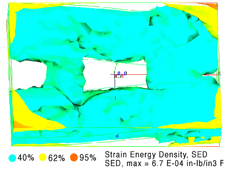
Figure 2. Carbon/Epoxy plain weave - thermal loading - SED.
It is interesting to see the effect of the material system not only on the magnitude of the maximum SED but the also on the location of the maximum SED. As shown in Fig. 3, the maximum value of SED (and local stress) exist at the centerline of the transverse yarns since for this particular geometry, the transverse yarns within the RVE are shorter than the corresponding axial yarns. This result suggests that failure in a glass/epoxy system, Fig. 3, will initiate in a yarn whereas failure in a carbon/epoxy system, Fig. 2, will initiate in a polymer region. Thus we can readily see that the differences in elastic moduli and coefficients of thermal expansion of the two material systems can effect the failure mode.
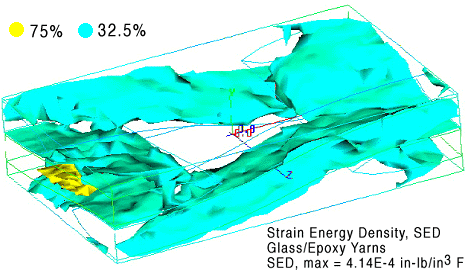
Figure 3. Glass/Epoxy plain weave - thermal loading - SED.
Mechanical loading is the primary load case for many structural composites including textiles. Figure 4 shows the SED contained within the same plain weave carbon/epoxy composite as discussed previously. In this case, a textile composite is subjected to uniform axial displacement. Here, the maximum values of SED are found in the axial (primary load bearing) yarns. As with the case of thermal loading, changes in the geometry can effect the value and location of the maximum values of strain, stress and SED.
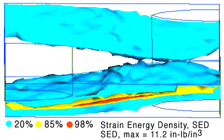
Figure 4. Carbon/Epoxy plain weave - axial loading - SED.
Static images of three dimensional translucent gradients of scalar properties have exceeded our visual abilities to interpret this data format. But, if these images are rotated in real time, it is possible for the "minds eye" to reconstruct the sequence of two dimensional images into a three dimensional volume. A small mpeg movie and large mpeg movie of a rotating RVE under a uniform axial displacement is provided here for viewing. For optimal viewing, download the mpeg movie onto your computer and play the sequence at a continuous rotation at about 15 frames / sec. Note that this RVE is composed of yarns with smaller aspect ratios (4:1 rather than the 8:1 and 10:1 seen in the previous figures) and thus has not only a large value of SED along the axial yarn centerline, but has an even larger SED located close to the transverse yarn cusps. In this model, the SED is composed of not only axial but also significant shear stress and strain components.
Another example of visualizing scalar gradients related to polymer composite fabrication and cure is the research of MacRae et al. [3]. In this simulation a variety of scalar properties were simulated and visualized. Figures and animations below show gradients in flow front gradients. Here the designer can gain insight into how the gradient of the property relates to the complex polymer composite structure and the visual tool that was used during the fabrication process. Figure 5 represents a stringer panel simulated during the cure process. The colored regions detail the flow front from 0 to 22 minutes into the processing cycle.
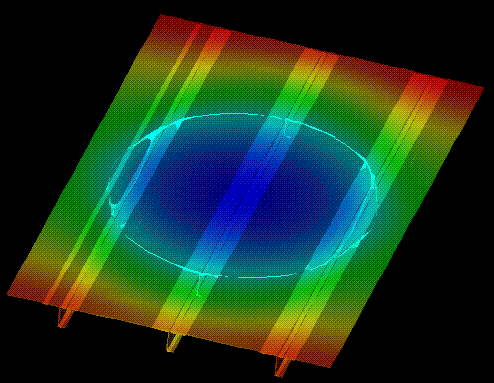
Figure 5. Flow front in graphite/epoxy stringer panel Ref. [3].
This sequence shows the moving resin flow front during the resin film infusion processing of the same blade stiffened panel shown in Fig. 5. The colored mesh, Fig. 6, represents time where the flow fron is highlighted. Illustration of the resin film movement allows for accurate verification and risk assessment of the tooling and processing parameters.
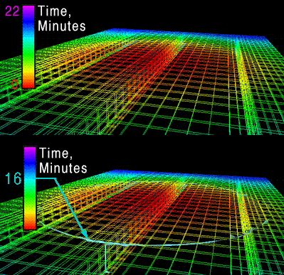
Figure 6. Two frames from a Mpeg movie showing the resin flow front movement through a panel where the flow front is highlighted.
Because these cure properties can coexist during the cure cycle there is an opportunity for the materials researcher to study how these properties interact with respect to unique and often complex panel configurations. Obviously these same images and animations can also be used to present the model simulation results.
These last two examples clearly show that visualization of scalar properties provides us with some interesting results. Additional information can be obtained if stress tensor distributions are included in the visual analysis.
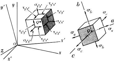
The components of any second order tensor can be reduced to an eigenvalue problem and visualized as a quadric surface, see Frederick and Chang [4]. Second order tensors can be used to represent the state of stress and strain in Lagrangian space or strain rate in Eulerian space. The components of a second order stress tensor can be written in a more familiar matrix format where it is easy to show that each matrix term is a vector component acting on the differential element shown in Fig. 7.
The second order stress tensor is transformed into an eigenvalue-eigenvector problem where tensor notation is used instead of matrices because of its notational brevity. For the reader who is more familiar with the matrix approach, any standard text on deformable bodies can be used.
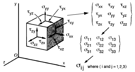
Figure 7. Stress tensor components shown on differential element.
(1)
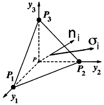
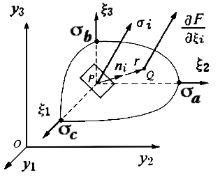
Figure 8. Stress vector and plane normal at an arbitrary orientation.
If the first order stress tensor (vector) and the unit vector normal to the plane (P1, P2, P3) in Fig. 8, shown above, have the same direction cosines then another relationship exists,
(2)
and this special case is referred to as a principal direction where the magnitude of this stress is called a principal stress. Substituting and rearranging indices.
(3) and (4)
where the symbol "delta" subscripted with i and j is a Kronecker delta or the identity matrix.
Considering Eqn. (4) and the orthogonality conditions, there are four equations with four unknowns. Equation (4) becomes an eigenvalue problem which can be rewritten here in a more familiar matrix notation,
(5)
where the stress scalars along the diagonal are the three eigenvalues (principal stresses) and the column vector are the eigenvectors (direction cosines: "orientations" of the principal stress state). When the differential element shown in Fig. 7 is rotated into the principal stress state the normal stresses become maximum and minimum and the shear stresses go to zero. This is shown on the cube to the right in Fig. 9.
To avoid a trivial solution, the determinant of the coefficient matrix in eqn (5) must be zero. This is written below in both tensor and matrix notation,
(6) and (7)
The eigenvalues can also be determined by expanding the determinate into a characteristic equation and solving for its roots. Either the roots or the eigenvalues together with the principal directions can be visualized as a quadric surface (elliptical glyph) whose major and minor axis lengths are the eigenvalues while the orientation of these axes (a,b,c) represent the eigenvectors. Frederick and Chang [4] outline several interesting properties of this stress tensor quadric.
(8)
Several other researchers [5, 6, 7, 8, 9] have demonstrated the usefulness of second order tensor glyphs is shown in the next section. In all these studies the glyphs revealed information that went beyond the initial physical understanding of the problem. Hence these studies demonstrated how glyphs provided insight that went beyond the traditional use of graphics, namely: graphics for presentation only. In the final section the authors show how these same ideas can be extended to higher order tensors and tensor equations where visual invariance can be used to extract simple relationships.
Haber [5] demonstrated how clusters of stress tensor glyphs could be used to study the singular stresses in the region of a moving crack in a solid. The following shows an array of principal stress glyphs near one of two crack tips, see Fig. 11, where stress tensor glyphs are combined with visualizing gradients in scalar properties of log(strain energy density) and Sqrt(kinetic energy) near the tip of a moving crack.
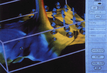
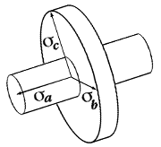
Notice that unlike the quadric surface glyphs, this glyph's shape is that of a simple rod and an elliptical disk. Although the quadric surface reveals additional information about the direction of the stress vector in a particular direction, Haber's glyphs are better suited to reveal magnitudes of the principal stress state. The shape shown below, Fig. 12, is more easily recognized for illustrating the major and minor axes which represent the eigenvalues or principal stress. The orientation of the glyph represents the direction (eigenvectors) of the principal stress state.
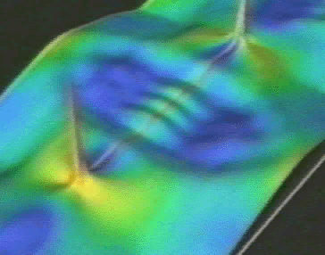
This visual tool reveals other interesting results such as interference patterns at the center of a plate caused by circular stress waves emanating from the two crack tips. Here the stress tensor glyphs have been removed.
An animated movie of Fig. 13, Ref. [6] ( MPEG Movie: 1.2Mb,141 frames ), displays the simulation - visualization results of two crack tips growing away from the center of the plate and shows the development of this interesting interference pattern. This stress wave interaction provided an explanation of the irregularities observed in the dynamic stress intensity factors.
The numerical solution to this fracture mechanics problem provided the raw data from which the stress tensor glyphs were created. Although these glyphs were observed to move over large distances with time, it is interesting to note that the deformation field is not Eulerian but Lagrangian.
Many problems in continuum mechanics emphasize continuous changes in tensor properties: such as the comoving derivative of a property associated with a fluid particle moving through a fluid in Eulerian space or continuous lines of principal stress in a solid where the deformation field is defined in Lagrangian space. Hence an alternate approach has been taken by Delmarcelle, Hesselink and Helman [7,8] where a continuous glyph is constructed to show a continuum of stresses.
In Fig. 14 the center of the two glyph tubes propagate upward along trajectories or lines that represent the direction (eigenvector) of the largest compressive stress. In this figure the color represents the magnitude of the largest compressive stress (the minor eigenvalue). The shape of the tube represents the magnitudes of the other two eigenvalues. Similar trajectories near the bottom of the figure for the other two eigenvectors take a shape that is everywhere perpendicular to the most compressive stress. These flattened tubes show that one of the eigenvalues must be close to zero.
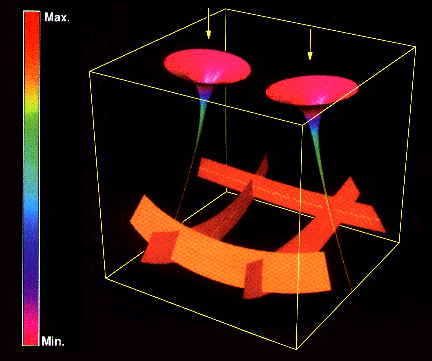
Figure 14. Elastic-stress tensor field in a solid induced by two compressive forces applied at the top surface, Refs. [7,8].
The next figure, Fig. 15, shows how the shape of the tubes in Fig. 14 change if an additional tension force is applied at the top surface (the exact location is not specified) Ref. [7,8]. The shape of these glyphs are shown to change with increasing tension force (a) -> (b) -> (c) -> (d).
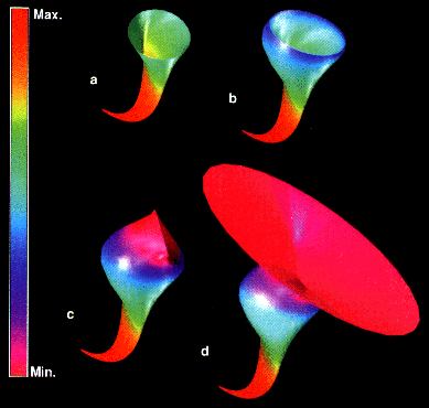
Figure 15. Elastic-stress tensor field glyphs shape changed by additional tension surface force. Glyph (c) shows that one of the principal stress is zero, Refs. [7,8]
In this example the magnitude of the compressive principal stress was mapped as color on the continuous stress tensor glyph. Many other combinations are discussed in Ref. [7,8].
Moore, Schorn and Moore [9] use Reynolds stresses to study turbulent flow. The stress tensor components are written here as a dyadic product which is equivalent to a tensor outer product of the fluctuating velocities (u, v, w).
(9)
Once the principal directions are determined, the principal components of the Reynolds stress tensor are found by transforming the fluctuating velocity components,
(10)
where the repeated indices "i" implies summation and the subscript "n" on P is not an index but implies principal directions. The dyadic product is used again to create the components of the Reynolds stress tensor but now in the principal stress state.
(11)
A new glyph can now be created by mapping this relationship into a cube with the unit vector (dx, dy, dz), where Sqrt ( dx**2 + dy**2 + dz**2 ) = 1.
(12)
As shown in Fig. 16 the resulting glyph is peanut shaped. Unlike the quadric surface the largest principal stress corresponds to the largest dimension and unlike the Haber glyph the exaggerated curvature of the peanut shape emphasizes the anisotropy. To emphasize the shape of this three dimensional glyph, Moore, Schorn and Moore [9] map contours of constant normal stress onto the glyph surface.
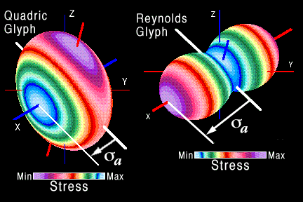
Figure 16. Comparison of the Reynolds stress tensor glyph with a quadric surface, Ref. [9].
The comparison in Fig. 16 demonstrates that the shape of the quadric surface does not accurately represent the eigenvalues because the geometry is used instead to represent the directions of the normal stress vector: property (i) of Fig. 10, the magnitude of the normal stress is inversely proportional to the square of the glyph dimensions along the principal axes. The Reynolds stress glyph more accurately shows the magnitude of the principal stress and magnitude of the normal stress by contours which are superposed onto the glyph's surface. The directions of the normal stress cannot be visualized on the Reynolds glyph. This tradeoff between showing magnitudes of principal stresses or directions of the stress vector is unavoidable. The choice of glyphs depends on emphasis of the researcher. With a flexible visual tool each researcher can taylor a glyph to emphasize the property of interest.
More information is obtained when using these glyphs in a distributed format as compared with previous methods using contour lines and vectors. These two visual methods are compared in Fig. 17 which is a composite of Fig. 2 and Fig. 8 taken from Ref. [9]. Larger image format is provided here for Fig. 17 taken from Ref. [9].
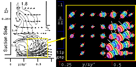
Figure 17. Comparison of Reynolds stress tensor glyphs with contour lines, Fig. 2 (left) and Fig. 8 (right) taken from Ref. [9].
Research continues on developing the Reynolds stress glyph at http://cmpendia.me.vt.edu/glyph/.
Glyphs can also be used to better understand higher order tensors. In particular, fourth order stiffness tensors can also be represented by simple glyphs. Several studies [10, 12, 13] of waves propagating in anisotropic material systems use Christoffel's equation to study the symmetries of propagating waves in different crystal class symmetries.
(13)
Again the eigenvalue problem is encountered where the eigenvalues are the wave speeds, v, and the eigenvectors are the particle vibration directions of Eqn. (13). Figure 18 shows all possible eigenvalues mapped into a continuous surface by prescribing all possible directions of a propagating wave. Here the wave propagation direction is denoted by the two wave vectors (indices i and j) that are contracted with the fourth order stiffness tensor, Cijkl. The eigenvectors which are physically the particle displacement vibration direction cosines (color: black-longitudinal and white-transverse) are mapped back onto the eigenvalue surface. Hence the relationship between the eigenvalues and their corresponding eigenvectors can be seen at every point. The spin properties of the displacement fields can also be seen as the singularities are approached along cones of internal conical refraction. It is through these singularities that wave surfaces can interconnect into single continuous wave surface (homotopic function (3.7Mb)) , Ledbetter and Kriz [10].
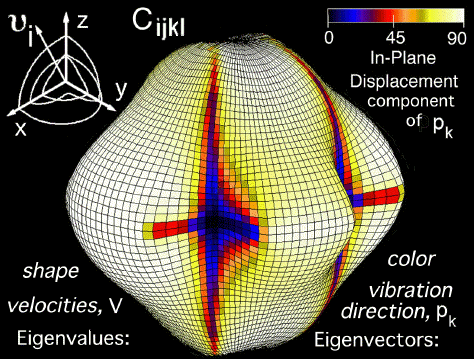
Figure 18. Fourth order stiffness tensor glyph for a single crystal of Calcium Formate (orthorhombic symmetry). Shape of surface maps the wave velocity for the fastest of the two quasi-transverse waves, Ref. [10]. NCSA's Polyview software, Ref. [11], maps the particle vibration directions onto the glyph surface as color: Black-longitudinal, White-transverse.
The reader interested in the tensor approach to this dynamic problem is encouraged to study references [10, 12, 13]. For the reader only interested in the previous example of the principal stress state, it is not difficult to show that Eqn. (13), reduces to Eqn. (4),
(4)
This is accomplished by a double contraction of the direction cosine tensor with the fourth order stiffness tensor. If we let
(14) and (15)
and
(16)
then we obtain the same tensor equation that defines the stress quadric,
(17)
except the term contracted with the fourth order stiffness tensor in Eqn. (14) is not just a simple second order tensor but derives its properties from a higher order tensor and hence enjoys a much richer surface topology then the simple stress quadric shown Fig. 18. Indeed the shape (eigenvalues) and colors (eigenvectors) iconically characterize all of the components of the fourth order stiffness tensor, Cijkl .
Sixth order tensors associated with the strain cubed terms of the strain energy density function can also be visualized by modifying Eqn. (13) to include the effect of load induced anisotropy. This problem is also an eigenvalue problem but now with sixth order tensors, see Ref. [14]. With an applied load, the resulting glyph in Fig. 18 should deviate from a symmetric shape. This shape change not only represents a change in elastic anisotropy but should also show the viewer the load direction.
There are many more examples of how other physical parameters effect the elastic fourth order stiffness tensor. With this visual method, materials researchers can now study and characterize how various physical parameters effect material anisotropy. Like the stress tensor glyphs in Fig. 11 and 17 it is also possible to view a distribution of fourth and higher order tensors in a continuum. This continuum of tensor properties leads us to think about extending these ideas to tensor equations.
Often more than one scalar function shares the same space. For example, pressure and temperature can simultaneously exist within the same region. Because only one color gradient can be seen within this region it is not possible to view more than one scalar function at a give time. However with new graphical features we can extend the previous method to observe more than one function in the same parametric space and hence test for the existence of these functions.
This method can be verified by including more than four parameters. For example it is possible to cognitively compare seven properties (P1, P2, P3, P4, P5, P6, and P7) in the same compressed visual space where four of the seven properties P1, P2, P3 and P4 are chosen as independent variables (not necessarily coordinate space and time). Hence this method provides a common basis from which to test for the existence of relationships between the remaining properties P5, P6, and P7. The procedure can be explained with a schematic drawing in Fig 19: the first three parameters P1, P2 and P3 are independent (orthogonal) variables that are visually defined as perpendicular axes in Fig. 19. The fourth property is reserved as another independent variable, e.g. P4 = time, that is uniform everywhere but cannot be drawn as the orthogonal fourth axis. The task remains to find relationships, if any, of the remaining properties P5, P6, and P7 that must all be functions of P1, P2, P3, and P4. For the simplest case this method can be reduced to a single function, where P4 is assumed to be constant everywhere. Of course this method can also be generalized to more than three functions P8, P9, ......., Pn where n is the viewers cognitive limit.
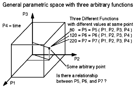
Figure 19. General parametric space with three arbitrary functions.
It is possible to see the full three-dimensional (3-D) gradient of either P5, P6, or P7 by using a translucent voxel element and mapping the entire region as a single continuous function. Often these 3-D gradients can only be understood when viewing the volume by a smooth and continuous rotation. This rotating voxel image is excellent for comparison but lacks the quantitative information format required in most applications. This trade-off between using qualitative and quantitative visual formats is discussed by Tufte, Ref. [15]. Tufte uses the example of advances in printing technology that occurred during the late eighteenth century when graphs began to supplement tables of numbers as a means of data presentation. Similarly in the last five years access to new graphic software has created another technology shift that not only influences the way we present information but also in the way we think about our functions. The effect of voxel imaging in some cases yields dramatic results, especially when the function is continuous with several contrasting regions.
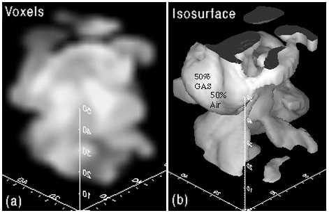
Figure 20. Volume visualization simulation of gas-air mixing: CM-2 computer at Naval Research Labs, Ref. [16]: (a) translucent voxel volume, (b) single isosurface.
Isosurfaces in Fig. 20b show only one ( "iso" ) concentration of gas, e.g. 50%, as a 3-D structure (surface) and is a more quantitative measure of the gas-air mixture. It would be possible to show this surface growing-shrinking as the value for percentage of gas increased-decreased. This would also show a gradient but only for small variations around 50%.
The voxels in Fig. 20a show a continuous gas-air gradation where this three-dimensional structure can only be seen if rotated: Mpeg movie (The movie may not play smoothly over the network. The viewer is encouraged to save this image sequence as a movie and play the movie at 15 frames / second on his/her own machine.) This type of graphic is less quantitative but gives a more qualitative measure of the gradient of a scalar function where the independent variables P1, P2 and P3 are (x,y,z) coordinate space and the fourth independent variable, P4 (time), is held constant. It is also possible to view changes in this 3-D gradient with time by letting the structure change with time as it rotates: a change in time corresponds to a change in rotation angle. Such a movie would allow the viewer to observe 4-D gradients. Larger number of independent variables are possible by creating slider bars or dials that can be changed interactively as the 4-D image rotates. Hence it is possible to create a 5-D visual gradient.
Rotating voxel images demonstrate the cognitive analytic power of the "mind's eye": that is, even elaborate and expensive computer tomography systems cannot accomplish the same analytical-numerical 3-D reconstruction of a rotating volume as fast as the human mind. Indeed our minds provide us with the ability to reconstruct 3-D, 4-D, 5-D, .... n-D images effortlessly where "n" is the cognitive limit of the viewer. Because this process is effortless, history shows that these new "easier" visual techniques are not at first well received. Tufte [15] points out that even though technology existed in the late eighteenth century to print graphs of complex functions, scientific archival journals continued to publish functions in a tabular format only. Graphs were considered not only inaccurate but with the addition of graphs almost anyone could understand the idea of a function.
Although the rotating voxel volume format allows the "mind's eye" to extract 3-D gradients, it is limited because only one function can be studied. To study the relationship between three functions P5, P6, and P7 that coexist in Fig. 16, another visual method must be created. This alternate visual method starts at some arbitrary point where each function P5, P6 and P7 can have unique values: P5 = 80, P6 = 120, and P7 = 220 respectively, see Fig. 19. Units are intentionally not shown. Obviously these values can change at adjacent points. This is the simplest idea of a gradient. Although all possible values for all three functions can not be seen in the same region, a quantitative isosurface can be seen for each function as a separate shaded surface. Imagine that it is possible to interactively change the isosurface value in Fig. 20b and instantaneously observe the corresponding change in shape. Then it is possible to deduce the gradient, but only in that immediate region. An animation could be effectively used here to demonstrate gradient changes in a particular region of interest. If this property were fluid pressure for example we could then envision the direction of flow by locating the region with the largest gradient in pressure: surfaces closest together.
Although it is tempting, and highly recommended, to think of the physics during the construction of any visual method, the method developed here does not address any particular physical problem, in the interest of developing this method as a general method. The reader can then take this general method and apply it to specific applications. Hence the method developed here can be used with any arbitrary 3-D numerical data set with three scalar properties. Two of the three properties are drawn as two unique intersecting isosurfaces as shown in Fig. 21. If the surfaces do not intersect then there can be no relationship between functions P5 and P6. If the surfaces intersect, then there is an opportunity to investigate further if this relationship is linearly proportional or inversely proportional.
It is important to note that this method does not require determining each function P5, P6, and P7 by a curve fitting method. In fact the relationship between P5, P6, and P7 can be determined without knowing anything about the functions themselves. Hence we can avoid curve fitting these functions and our attention focuses on how these arbitrary shapes (arbitrary functions) relate to each other.
Because these functions are arbitrary, it is convenient to choose P5 and P6 as simple spherical functions whose isosurfaces are conveniently viewed as intersecting nonconcentric spheres, as shown in Fig. 21. If P7 is an independent function not related to P5 or P6 then P7 can be mapped as a color on P6 and it is possible to view these arbitrary gradients in P7 where P6 is observed to be constant. Conversely, it is possible to observe that P7 is a constant where P5 and P6 intersect because a constant color (P7) is observed adjacent to the intersecting P5 and P6 surfaces, as shown in Fig. 22. Note that because small changes in color (gradient) are sometime impossible to see, it is necessary to show the color gradient by a third surface intersecting near the intersection of P5 and P6. If arbitrary variations in P5 or P6 yield similar results then P5, P6, and P7 are either proportional or inversely proportional to each other.
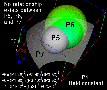
Figure. 21. No relationship exists between P5, P6, P7. Note here a translucent surface (P7) is drawn intersecting the P5, and P6 isosurfaces to aid the observer in seeing small changes in the color gradient mapped onto the P6 isosurface. These small changes in color gradient could be observed by modifying the color table and the P7 surface can then be eliminated.
In Figs. 21 and 22, parameter P4 (i.e. time) is held constant and P5, P6, and P7 are scaled as ( min=1 and max=256 ) and the range for P1,P2, and P3:
                  1 < P1 < 120,
                  1 < P2 < 80,
                  1 < P3 < 100.
To determine this function the following relationship is assumed:
( P5 ) ( P6 ) ( P7 ) = constant (18)
This relationship is possible if we observe a constant color (P7) at the intersection of P5 and P6 surfaces but it is only one of three possible relationships.
     ( P5 )  ( P6 )  ( P7 )  =  constant,
     ( P5 )  ( P6 )   =   constant  (P7),
     ( P5 )    =    constant  (P6)  (P7)
Each of these functions would show a constant color (P7) at the P5-P6 intersection. With additional information this method can be used to check if an assumed function is correct. For example:
If P6 is held fixed and P5's isosurface is arbitrarily increased it is possible to observe a corresponding linear increase in the intersecting color for P7 then it is possible to concluded that:
(P5) (P6) = constant (P7) where P6 = constant and P4 = constant (19)
is the correct relationship.
Now if P5 is held fixed and P6 is increased about some arbitrary value and the image shows a corresponding decrease in P7 by some constant, therefore it is possible to conclude that:
(P5) = constant (P6) (P7) where P4 = constant (20)
which is the correct relationship over the entire parametric space. Finally if the three parameters P1, P2, and P3 are fixed and only P4 is changed, then it is possible to observe that the same visual patterns occur for any arbitrary value of P4. Therefore the final conclusion is this method shows:
(P5) / [ (P6) (P7) ] = constant, for all P1, P2, P3, and P4. (21)
exists everywhere arbitrarily.
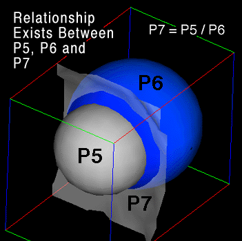
Figure 22 Simple proportional and inversely proportional relationships exist for P5, P6, and P7. Note here P7 is drawn as a translucent isosurface, so that the observer can better view the small changes in color for the P7 property.
Here, the idea of arbitrariness is used in the same sense as it is used in continuum mechanics when confirming the existence of a tensor equation. Equation (21) is a simple zeroth order tensor equation where, not only are the scalar parameters themselves invariant to arbitrary coordinate transformations, but the scalar equation is also invariant to any arbitrary transformation. This same requirement for mathematical invariance is also the fundamental idea of a physical law. That is, the parameters P5, P6, and P7 must always satisfy the same relationship independent of any arbitrary transformation of parameters P1, P2, P3, or P4. This same visual paradigm of invariance can be extended to higher order tensor equations, as was shown is section 4 as an eigenvalue problem solution with fourth order tensors.
Such simple scalar functions, Eqn. (21), commonly occur in nature. For example let P1, P2, P3 be coordinate space and P4 = time, and let P5, P6, and P7 be pressure, density, and temperature functions respectively, then the constant becomes the gas constant, R, (see Fig. 23). Again it is possible to enhance the color adjacent to the surface intersection. An expanded picture of Fig. 23 shows how exiting visualizaiton software tools can be used to create an interactive environment to detect and extract functions. Note that this method confirms the existence of such simple functions without curve fitting the functions P5, P6, and P7 to parametric space: We did not need to calculate the function for each of the irregular surfaces in Fig. 23 to verify the relationship between P5, P6, and P7.
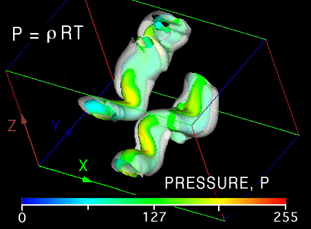
Figure 23. Extracting the gas law: a simple scalar zeroth order tensor equation.
With this method it is possible to successfully find many more complex functions. In all cases, just as in finding solutions to differential equations, the reader must guess at possible solutions. This guess can then be visually confirmed by constructing the necessary visual paradigm using existing visualization software packages or constructing other modules that provide additional unique features required for the visual confirmation. Of course only significant functional components will be detected and extracted much like the dominant terms in a series solution. Mentally the observer first sees a pattern related to the function and can then deduce the function mathematically. Hence the pattern of a function occurs first and becomes the cognitive mechanism that allows the investigator to confirm the existence of suspected functional relationships. Again the computer is used to perform tedious tasks of drawing a complex graphical representation of the idea where in the past only a few gifted scientists demonstrated an inherent ability to perform this same process psychically.
"What I really try to do is bring birth to clarity, which is really a half-assedly thought-out-pictorial semi-vision thing. I try to get the pictures clearer, but in the end the mathematics can take over and be more efficient in communicating the idea of the picture. In certain particular problems that I have done it was necessary to continue the development of the picture as the method before the mathematics could be really done." Richard Feynman in an interview by Silvan S. Schweber, Ref. [17].
![]() Return to VT Work Shop Presentations
Return to VT Work Shop Presentations
 Return to Visualization Home Page