 |
(35) |
Ronald D. Kriz, Associate Professor
Engineering Science and Mechanics
Virginia Polytechnic Institute and State University
Blacksburg, Virginia 24061
To include all components of a fourth order stiffness tensor in a geometric representation of anisotropy requires we look closer at the equations of motion for an anisotropic solid (dynamic mechanical behavior). Here our objective is to look at a spherical disturbance such as a dilitational pulse that expands equally in all directions: invoking Huygen's principal the reader can envision a very small plane wave exists on the surface of a very small sphere in the center of an anisotropic crystal. One can simply imagine that from Huygen's principal each of these plane waves travels in a specific direction, direction cosines, νi, at a speed that corresponds to elastic properties unique to the same direction. Hence, plane waves traveling in different directions will travel at different speeds and the continuous collection of all of these plane waves, although initially a sphere, soon deviates into a nonspherical shape simply because plane waves will travel faster in stiffer directions and slower in less stiff directions. This idea was modeled and simulated for a highly anisotropic Calcium-Formate crystal, "Spherical Wave Simulation in 2-D Anisotropic Media". The three-dimensional wave surface for a Calcium-Formate crystal was first plotted in Ref.[13]. We will show that this wave surface topology does indeed uniquely describe the complete set of components of the fourth order stiffness tensor. These resulting geometries are now being used as new sub-classification schemes within orthorhombic symmetry, Ref.[14].
First we start with the equations of motion for a continuum.
|
|
(35) |
Recall equation (17)
 |
(17) |
and substitute the strain-displacement relationship, equation (7),
 |
(7) |
into equation (17) yields
 |
(36) |
Recall that the strain tensor is symmetric which further reduces equation (36).
 |
(37) |
Substitituting equation (37) into equation (35) yields the equation of motion in terms of displacements.
 |
(38) |
This equation can be further reduced if we assume the material is homogeneous.
 |
(39) |
With this simplification equation (38) reduces to a form where we can now assume a solution for displacement and substitute it into this equation.
 |
(40) |
Let us assume a small plane wave periodic disturbance, see Figure 17.
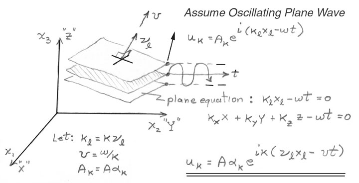
Figure 17. Mathematical model for a plane wave disturbance: oscillating plane written in exponential format in terms of wave velocity, v, propagation direction, νl, and particle vibration direction, αk
The periodic displacement shown in Figure 17 uses an exponential functional form instead of sines and cosines because it will be easier to differentiate. The reader can envision a plane wave in Figure 17 where the wave number coefficients, ki, are terms used to define a plane (this will perhaps require a review of basic descriptive geometry in freshman calculus) and the circular frequency, ω, when multiplied by time, t, replaces the constant for a plane with a term which models the oscillatory motion of that plane.
 |
(41) |
The terms in equation (41) can be replaced with wave velocity, v, and direction cosines of the propagation direction, νi which will allow the reader to interpret the results of this particular eigen-problem in a more meaningful way.
 |
(42) |
Substituting equation (42) into equation (40) and after much manipulation, equation (40) reduces to an eigen-value problem which is written below in both tensor and matrix notation.
| tensor equation: |
 |
(43) |
matrix equation:
 |
(43) |
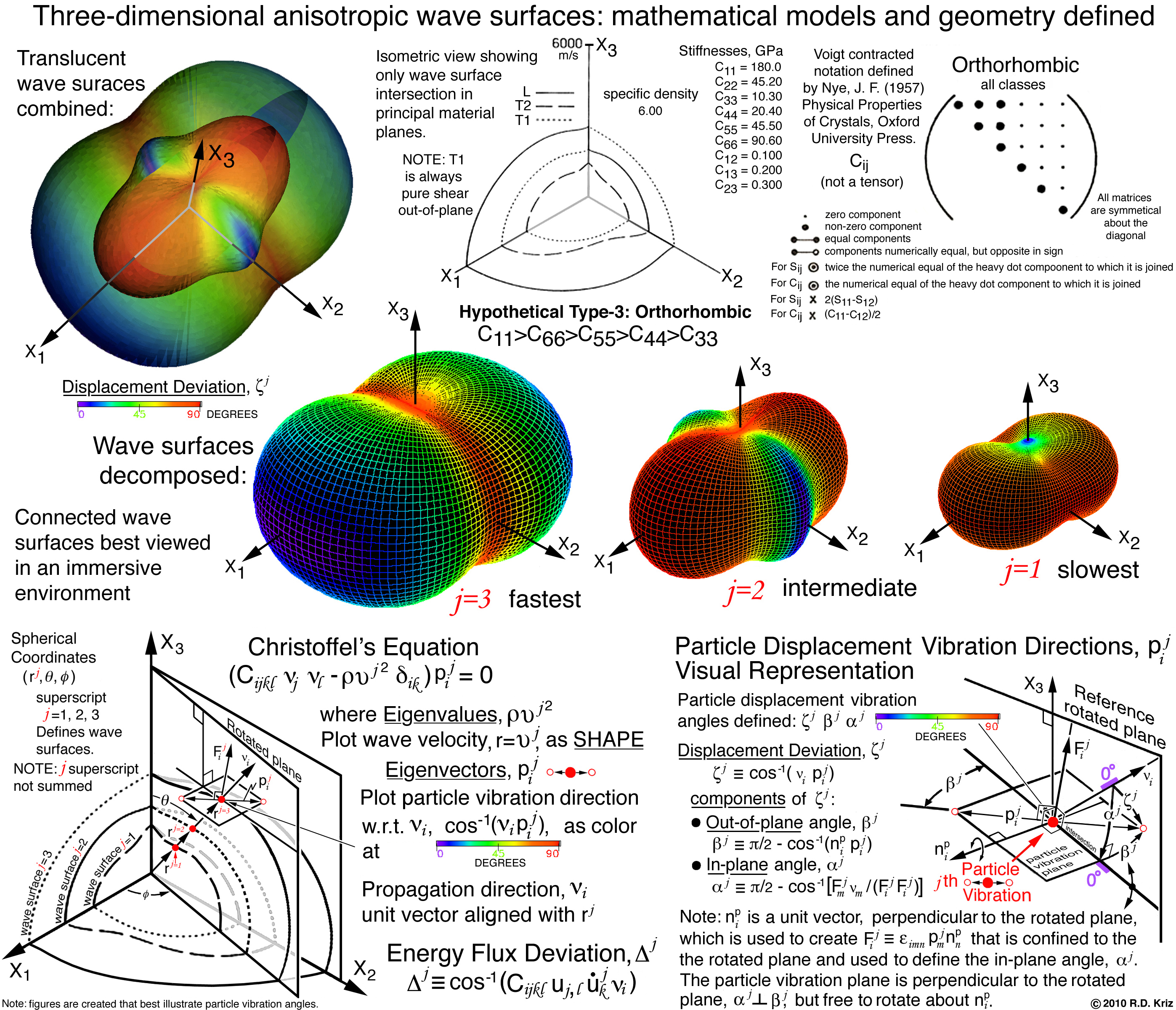
If we use the matrix form of equation (43) it is easier to see that the velocity terms along the diagonal, ρv2, are the eigen-values and the displacement direction cosines, αi are the eigen-vectors. Closer examination of the solution to this particular eigen-value problem reveals that both the eigen-values and eigen-vectors can only be functions of ALL stiffness tensor components for an assigned propagation direction, νi. Hence we conclude that if we solve for eigen-values (wave speeds) in all possible propagation directions, νi and connect points to form a continuous surface, this would generate a 3-D shape of wave speed for each eigenvalue. Since there are three eigen-values, equation (43) predicts three wave surfaces: 1) longitudinal which is usually the fastest and observed as the largest shapes, and 2) two different shear ("transverse") waves which are usually slower and consequently observed as smaller shapes. The eigen-vectors which are particle vibration direction cosines (0 to 90 degrees) can be mapped onto the eigen-value surfaces as color. Hence the color would reveal the type of wave: longitudinal (0-degrees i.e. purple) and transverse (90-degrees i.e. red) where green would indicate a mode transition from longitudinal to transverse. With colors the observer can quickly determine the wave type and discover possible mode transitions. Graphical definitions of these and other properties associated with this solution are given by the problem statement / updated statement.
Some obvious geometric features that correspond to anisotropy are: 1) stiffer directions map as a larger distance from the geometric center which would be seen as "bulges" and 2) less stiff directions map as smaller distances from the geometric center which would be seen as "depressions". Highly anisotropic materials would appear as significantly deviating from the isotropic spherical geometry. Graphite-Epoxy and Calcium-Formate exemplifies all of these features, see Figure 18 and Figure 19.
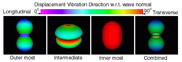
Figure 18. Wave surfaces predicted for Graphite-Epoxy, Hexagonal symmetry
NOTE: light-blue/green indicates a mode transition -- a very rare anisotropy
which
is only observed in Calcium-Formate, spruce-wood, and graphite/epoxy.
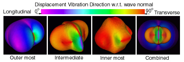
Figure 19. Wave surfaces predicted for Calcium-Formate, orthorhombic symmetry
NOTE: light-blue/green indicates a mode transition -- a very rare anisotropy
which
is only observed in Calcium-Formate, spruce-wood, and graphite/epoxy.
Figure 19 shows the solution of equation (43) for an orthorhombic fourth order stiffness tensor of Calcium-Formate, Ref.[13]. This particular tensor has a rare anisotropy that requires all three wave surfaces to connect into a single contiguous surface, see "combined" wave surface of Figure 19. A simple movie demonstrates both the connected surfaces and mode transitions previously described. The only other known material that exhibits this anisotropy (geometry) is Spruce wood. References [13-15] identify four possible geometries not previously known. With these geometries it is now possible to derive a subclassification scheme for orthorhombic anisotropy.
By studying the wave surface geometries it is also possible to study and compare elastic property anisotropy from isotropic to orthorhombic symmetry. Below is a table listing elastic material properties for each of these symmetries.
| Material: Stiffnesses GPa | Density gm/cm3 |
C11 | C22 | C33 | C44 | C55 | C66 | C12 | C13 | C23 |
|---|---|---|---|---|---|---|---|---|---|---|
| Staniless Steel (isotropic) / Update | 7.88 | 261.0 | 261.0 | 261.0 | 77.5 | 77.5 | 77.5 | 106.0 | 106.0 | 106.0 |
| Aluminum, (cubic) / Update | 2.70 | 108.0 | 108.0 | 108.0 | 28.0 | 28.0 | 28.0 | 62.0 | 62.0 | 62.0 |
| Zinc (hexagonal) / Update | 7.10 | 143.0 | 143.0 | 50.0 | 40.0 | 40.0 | 63.0 | 17.0 | 33.0 | 33.0 |
| Aligned Graphite/Epoxy (hexagonal) / Update | 1.61 | 14.5 | 14.5 | 160.0 | 7.07 | 7.07 | 3.62 | 7.26 | 5.53 | 5.53 |
| Tellurium Oxide (tetragonal) / Update | 4.99 | 55.7 | 55.7 | 106.0 | 26.5 | 26.5 | 65.9 | 51.2 | 21.8 | 21.8 |
|
Benzene (orthorhomibic Type-1)
/
Update
( C11, C22, C33 ) > ( C44, C55, C66 ) |
1.06 | 6.14 | 6.56 | 5.83 | 1.97 | 3.78 | 1.53 | 3.52 | 4.01 | 3.90 |
|
Calcium Formate (orthorhombic Type-2)
/
Update
( C11> C33> C 66> C22> C55> C 44 ) |
2.02 | 49.2 | 24.4 | 35.4 | 10.5 | 12.2 | 28.2 | 24.8 | 24.5 | 14.5 |
|
Hypothetical (orthorhombic Type-3)
/
Update
( C11> C66> C55> C22> C44> C33 ) |
6.00 | 180.0 | 45.2 | 10.3 | 20.4 | 45.5 | 90.6 | 0.100 | 0.200 | 0.300 |
|
Hypothetical (orthorhombic Type-4)
/
Update
( C11> C22> C66> C44> C55> C33 ) |
3.00 | 80.1 | 60.2 | 10.3 | 30.4 | 20.5 | 40.6 | 0.100 | 0.200 | 0.300 |
Figures below correspond to the last four orthorhombic symmetries and their corresponding elastic property inequality.
Figure 20. Examples of the four basic types of geometries and their corresponding
inequalities that can be used to subclassify within orthorhombic symmetry
The inequalities for each of the four types of orthorhombic symmetries are the necessary and sufficient condition that defines each unique geometry. These geometries and their corresponding inequalities can be used to create a subclassification scheme within orthorhombic symmetry. For those interested we have provided a graphical proof.
Other highly anisotropic materials such as graphite/epoxy can also significantly influence dynamic mechanical behavior. The section on Simulation and visualization of wave propagation in unidirectional graphite/epoxy composites Ref.s [16], [17], and [18], summarizes how unidirectional graphite/epoxy composites like Calcium Formate exhibit mode transitions but without resulting in a connected wave surface. Unlike Calcium Formate, which is a crystal, graphite/epoxy derives its anisotropy from its' constituent fiber and matrix properties (microscale), hence elastic properties at the microscale can signficantly influence anisotropy and dynamic mechanical behavior at the macroscale. For graphite/epoxy it can be shown that not only can anisotropy have a significant effect on dynamic mechanical behavior, see Figure 21, but degradation of either the fiber or matrix phase can preferentially alter the direction of the wave propagation from the initial undegraded state, see Figure 22. A section on simulation-visualization in unidirectional graphite/epoxy composites allows the reader to explore the influence of anisotropy on these and other possible dynamic mechanical behaviors using a small grid (30x60) or large grid (45x180) finite element grid model. For confirmation with an exact solution a simple isotropic one-dimensional model is provided here for the reader. Experimental confirmation of the accuracy of these physical based simulation models is given in Ref.[10] Figure 14, see Figure 23.
Figure 21. Schematic of simulation and
animation
summarizing
wave properties of a full field simulation.

Figure 22. Influence of preferential microscale elastic component
degragation on macroscale mechanical behavior.
Figure 23. Experimental confirmation of beam steering, Ref.[10] Figure 14.
The discussion above provides an excellent example of how elastic properties scale from the nanoscale (fiber transversely-isotropic nano-structure) to the microscale (transversley-isotropic unidirectional composite) and ultimately influence the dynamic mechanical behavior at the macroscale (beam steering and mode transitions). The diagram below illustrates how the wave length of a stress wave scales from the macro to the nano structures. Indeed the commponents of the elastic stiffness tensor are derived from the nanostructure of the atomic spacing.
Figure 24. Wave length and elastic properties scale from nano to macro.
Other sections on: 1) Visualization of Stress Waves in Elastic Solids and 2) Simulation and Visualization of Energy Waves Propagating in 2-D and 3-D Anisotropic Media, provide more information on how anisotropy controls dynamic mechanical behavior.
We have demonstrated that anisotropy in crystals like Calcium-Formate and undirectional composites like graphite/epoxy exhibit unusual dynamic and static mechanical behavior. As designers we can take advantage of this anisotropy. Because the elastic properties of graphite/epoxy can be tailored, engineers can design the material for the application instead of designing an application around fixed material properties. One popular method of exploiting the anisotropy of graphite/epoxy, in the design of a desired mechanical behavior, is to use laminate plate theory.